The Heritage Foundation’s Budget Blueprint for Fiscal Year 2022 proposes a combination of spending cuts and tax cuts to roll back the size, scope, and reach of the federal government to its proper role.REF Traditional budget scores apply proposed changes while assuming that macroeconomic variables, such as gross domestic product (GDP) and interest rates, remain unchanged. Dynamic scores use economic models to account for the likely effects that changes in tax rates and direct federal spending will have on the prices and quantities across several markets.
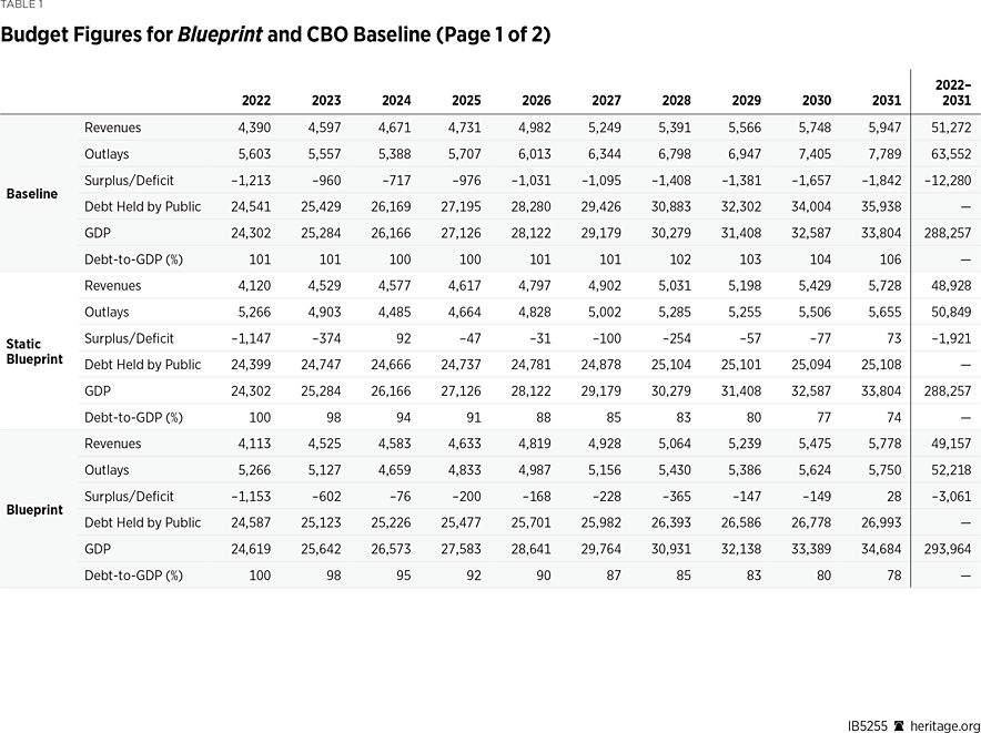
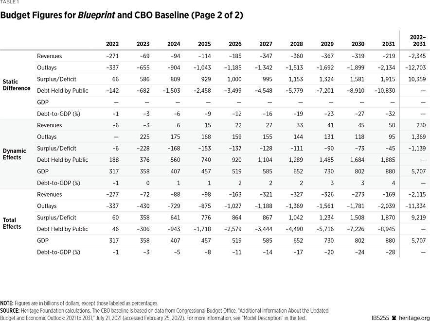
Incorporating macroeconomic effects in the Blueprint increases revenues and outlays relative to the static estimates. The increased revenues come from an increase in GDP, which is 2.6 percent higher by the end of the 10-year budget window from 2022 to 2031. The increased outlays are due to increases in the interest rate on government debt corresponding to the increase in output. In both the static and dynamic estimates, the net result of the Blueprint is significant reductions in outlays and revenues relative to the current-law baseline.
At the end of the 10-year window, debt held by the publicREF is about $1.9 trillion higher in the dynamic estimate than in the static estimate. Debt relative to GDP is slightly higher, reaching 77.8 percent in the dynamic estimate compared to 74.3 percent in the static estimate. In both Blueprint estimates, debt relative to GDP is significantly lower than the estimate in the baseline. While the dynamic estimate sees a slower reduction in the debt, it also recognizes the benefits of increased income: Over the 10-year window, GDP increases by $5.7 trillion.
The estimates for this edition of the Blueprint use an updated model from the version used in the fiscal year 2020 Blueprint.REF The current model is a computable general equilibrium (CGE) model. The CGE model is populated with households and firms who participate in markets. Their supply and demand curves are derived from forward-looking optimization problems, meaning that they respond to current and future changes in policy.REF Wages and interest rates adjust so that markets for labor and financial capital reach equilibrium along a balanced growth path. More details and a brief description of the solution procedure are presented at the end of this Issue Brief.
The neutral cost recovery for structures and the reduction of the corporate income tax rate in the Blueprint have the strongest effect on the economy. The tax cuts increase the after-tax return to capital, so firms want to invest more and seek to finance the investment from the savings of the household sector. In order to induce households to save more, the real returns to equity and debt must increase. Correspondingly, the government must pay higher interest rates to entice the private sector to hold its debt. Given the increase in the debt in the wake of the COVID-19 pandemic, outlays became more sensitive to increases in interest rates.
Reductions in income taxes and the increased investment combine to raise labor hours, the capital stock, and total output. The increased economic activity generates new revenue, partially offsetting the reduction in revenue from the rate cuts. The dynamic effects increase revenues by about 15 percent to 20 percent of the static cuts. The increase in revenues relative to the static estimate occurs despite a lower tax burden on the private sector. With the tax rates in the Blueprint, the federal government takes a smaller slice of a bigger economic pie.
Table 1 shows revenues, outlays, surpluses, debt, and GDP under model equivalentsREF of the Congressional Budget Office (CBO) baseline and the Blueprint’s proposals. The static estimate of the Blueprint’s proposals is calculated by applying the policies from the Blueprint and using the market prices and tax bases from the CBO baseline. Using model equivalents puts the different estimates on equal terms, allowing an apples-to-apples comparison of the static and dynamic effects, which are reported in the bottom half of Table 1.


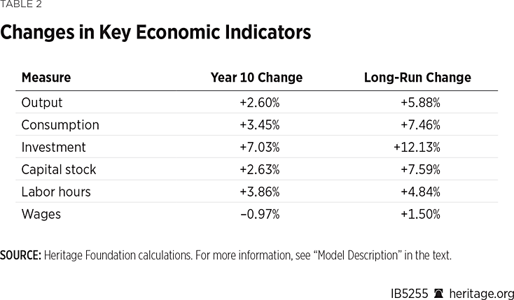
While debates over budgets often focus on the 10-year budget window, the proposed changes to the tax code in the Blueprint also have long-lasting effects. The transition to a new balanced growth path with a larger capital stock occurs over many years. Table 2 shows changes in key economic indicators estimated at the end of the 10-year window and over the long run at the new economic equilibrium.

In the new equilibrium, GDP is 5.88 percent higher than it would be under current law. Consumption, investment, capital, labor, and wages all continue to grow outside the 10-year window.
In the initial years, the cut in individual income taxes and the increased return to saving combine to increase labor supply, which pushes wages down relative to the model-equivalent baseline. However, wages rise over time as the larger capital stock makes workers more productive.
The years beyond the budget window also have important effects for transfer programs, such as Social Security and Medicare. Beyond the 10-year budget window, I assume in this Issue Brief that Congress leaves policy generally unchanged for 30 years, then cuts transfer payments by enough that debt slowly approaches a target relative to GDP.REF The baseline requires sharp cuts to transfer programs after 30 years. By starting the government on the path to stable debt earlier, the Blueprint avoids the sharp cuts to transfer programs to stop debt from exploding.REF
Readers should use caution when interpreting the results in this Issue Brief. The budget figures presented here use a format that facilitates comparison with other static estimates. The model that produces these estimates is simpler than the procedures that produce the static estimates in order to keep the computation of an equilibrium path manageable. Development to add more detail will continue with future iterations of the Blueprint.
However, readers should have confidence in the broad story of the dynamic effects produced by the model. Reducing taxes on capital increases the capital stock and GDP. Higher GDP recovers a portion of the revenue lost from the tax cut. Increased investment raises interest costs for the government, which slows down the rate of debt reduction.
While the dynamic effects likely give a more accurate estimate of the Blueprint’s proposals, both the static and dynamic estimates tell the same story. Tax cuts are paid for by spending cuts. Both revenues and outlays fall relative to the baseline. Debt-to-GDP falls relative to the baseline. However, the dynamic estimates provide information about a major benefit of reducing the size and scope of the federal government’s economic activity—higher incomes.
Using either the static or the dynamic estimate of the proposals in the Blueprint sets the federal government on the path to a stable level of debt and promotes prosperity through the private sector.
Model Description
The dynamic economic model used in this Issue Brief uses techniques similar to those used in a review paper by George Zodorow and John DiamondREF and a textbook by Burkhard Heer and Alfred Maussner.REF
The CGE model has a single representative household with utility that depends on consumption of a single composite good and leisure. The representative household has expenditures on the consumption good, purchases of equity stakes in firms, and purchases of debt issued by governments. Its income comes from providing labor to firms and governments at market wages, receiving dividends from firms’ earnings, receiving interest from government debt, and receiving transfer payments from governments. Given its budget, the household chooses consumption, labor hours, purchases of equity, and purchases of debt in order to maximize its lifetime utility.
There are two types of firms in the model: corporate and non-corporate. Firms choose to hire labor and choose an investment plan to maximize the value of the firm to existing shareholders. Firms are assumed to pay a constant fraction of their earnings as dividends. They issue equity to cover the cost of investment above and beyond retained earnings. Additionally, corporate firms are subject to the corporate tax rate, while non-corporate firms are not.
In order to change the capital stock, firms must face adjustment costs through forgone output (such as needing to shut down a factory in order to install upgraded machinery). The presence of adjustment costs means that firms make changes to the capital stock more slowly than if adjustment costs were absent.
There are two governments in the model: the federal government and the combined state and local government. Both governments raise revenue by levying seven types of taxes: taxes on (1) wages, (2) capital gains, (3) dividends, (4) interest, (5) corporate income, plus (6) payroll taxes for social benefits and (7) sales taxes on produced output. They spend money on purchases of the consumption good and lump-sum transfer payments to households. Value added by the governments is assumed to be a constant proportion of spending on the consumption good by governments, which raises real output, all else equal.
The model treats marginal and average tax rates separately. Marginal rates are taken directly from policy or taken as a dollar-weighted average of marginal rates when taxes have graduated brackets. Average tax rates are calibrated so that the model matches observed revenues relative to output when applied to tax bases calculated from the model.
The model is solved using the extended path method of Ray Fair and John Taylor.REF Agents are presumed to have perfect foresight over future policy. They solve for the equilibrium variables over a transition path ending at the long-run steady state. The estimates presented here consider a transition path of 150 years at an annual frequency.
The federal government must have a stable debt-to-output ratio in the long-run equilibrium. Since the proposed 10-year budget plans do not produce the necessary surpluses, nor does current law within the next 30 years, the model presumes that efforts to stabilize the debt start after 30 years. The government sets a target debt-to-output ratio and reduces the excess debt by 1 percent per year by reducing transfer payments to households.
Parker Sheppard, PhD, is Research Fellow for Dynamic Modeling and Simulations in the Center for Data Analysis, of the Institute for Economic Freedom, at The Heritage Foundation.


