Introduction
COVID-19 has been a crisis unparalleled by any other public health catastrophe in modern times. Shortly after being declared a global pandemic in March, the federal government and state governors throughout the country issued a variety of directives intended to quell the spread of the virus.REF As of March 5, 2021, having infected over 115 million people globally and claimed the lives of 2.5 million, it is imperative for lawmakers to understand how to more effectively combat the disease in the coming months, as well as better prepare for other potential crises that may come our way.REF
Fortunately, although there is still room for improvement, a plethora of data exist that can help public officials combat COVID-19 and prepare for future pandemics. This Special Report provides a statistical analysis of some of this data. In particular, we examine the spread of the disease throughout the country, the factors impacting mortality rates, behavioral responses across all 50 states, and the efficacy of the policies instituted to curb the spread of the virus. This analysis is based on data that is available and is not intended to establish causation in a medical sense. Regardless, our goal is to help elucidate how the disease has proliferated and how effective the mitigation policies instituted have been.
The Proliferation and Mortality of COVID-19
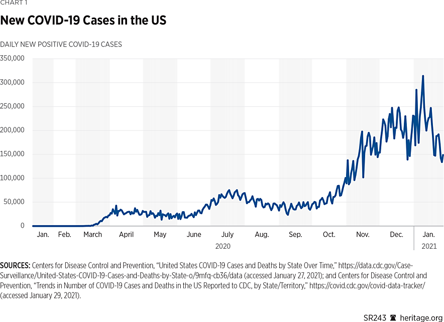
The United States has a population of more than 329 million people. Although it is still unclear exactly when the virus first came to the United States, the first reported case on American soil occurred on January 21, 2020, in Washington State.REF Cases and deaths quickly grew in the ensuing weeks and incurred several spikes over the course of the year. Chart 1 presents daily new COVID-19 cases in the United States as reported by the Centers for Disease Control and Prevention (CDC).REF
So far, COVID-19 has been responsible for over 25 million confirmed cases and over 430,000 deaths.REF As Chart 1 demonstrates, new COVID-19 cases have fluctuated during the past several months, with a recent spike occurring at the beginning of October.

Initially, a primary reason for many of the policy measures taken during the course of 2020, including shelter-in-place orders issued across all 50 states (and the District of Columbia), was to “flatten the curve” (prevent local hospitals from becoming overwhelmed) and to reduce mortality.REF Chart 2 depicts weekly COVID-19-associated hospitalizations across the United States.
As Chart 2 shows, the country incurred a dramatic increase in early COVID-19-related hospitalizations that started in mid-March. Increased hospitalization rates sparked fear of hospital beds being overrun in many areas of the country.REF After a moderate tapering, the country experienced a second wave starting in late June and a higher third wave in October. In late November, hospitals in some states were still reporting difficulty allocating resources to treat COVID-19 patients, despite the fact that officials had time to plan for excess patients.REF
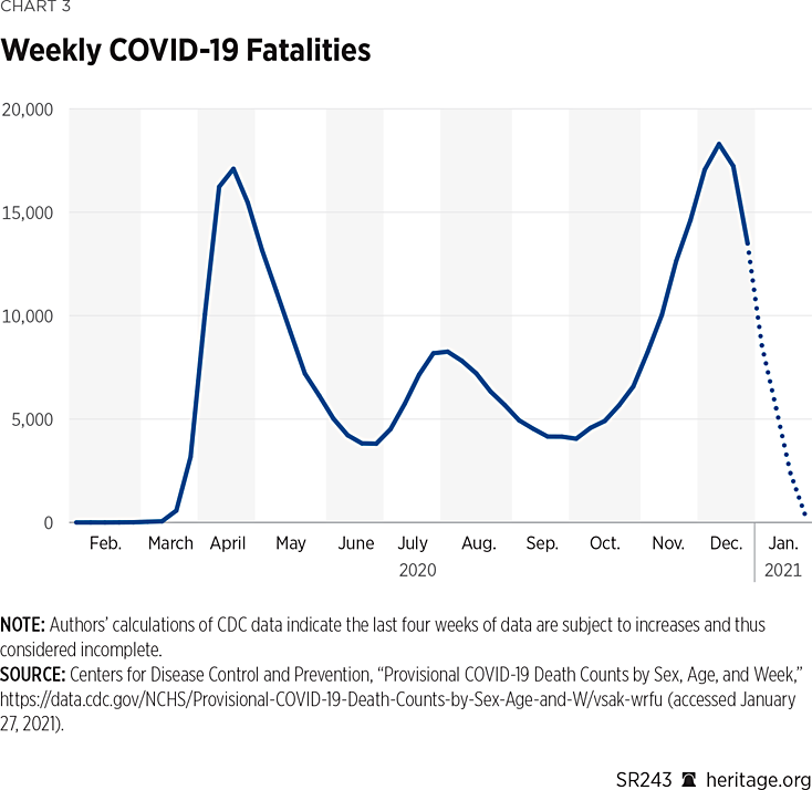
Regardless, most hospitals and state and local health officials have so far successfully handled these surges.REF As of January 30, 2021, the national intensive care unit (ICU) occupancy rate is about 76 percent, with six states having more than 85 percent of their beds occupied.REF Chart 3 depicts weekly COVID-19-associated deaths across the United States.
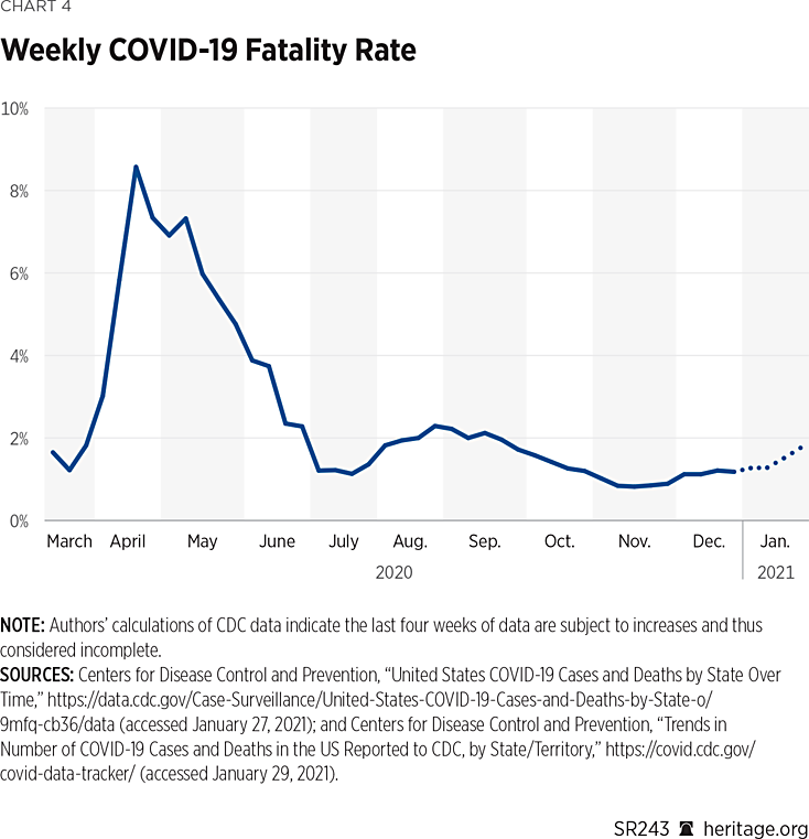
Specifically, Chart 3 shows the alarming and tragic spike in COVID-19 deaths that began after March 14, 2020, and reached a peak of 17,078 weekly deaths. The total numbers began to decline after April 18, before a second wave of deaths began in late June. The apex of this wave reached a weekly height of 8,178—52 percent lower than the initial spike. After October 1, a third wave of fatalities began. According to weekly CDC data depicted in Chart 4, however, the case–fatality ratio (ratio of fatalities to confirmed cases) has exhibited markedly different behavior over time. As Chart 4 illustrates, the case fatality rate (new fatalities divided by new cases) around the apex of the first wave in mid-April was almost 9 percent. The case fatality rate at the height of the second wave (in late July) was approximately 2 percent. If recent data holds true, due to more numerous reported infections and fewer fatalities, the height of the third wave will not likely rise above 2 percent. When one examines the hospitalization and mortality data amongst various age groups, however, disparities amongst cohorts become quite apparent.
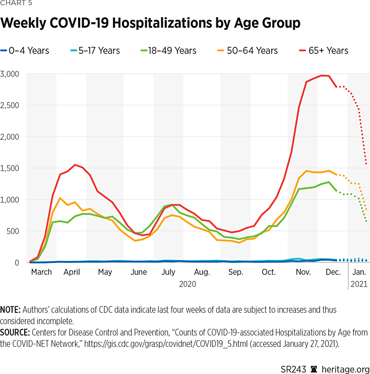
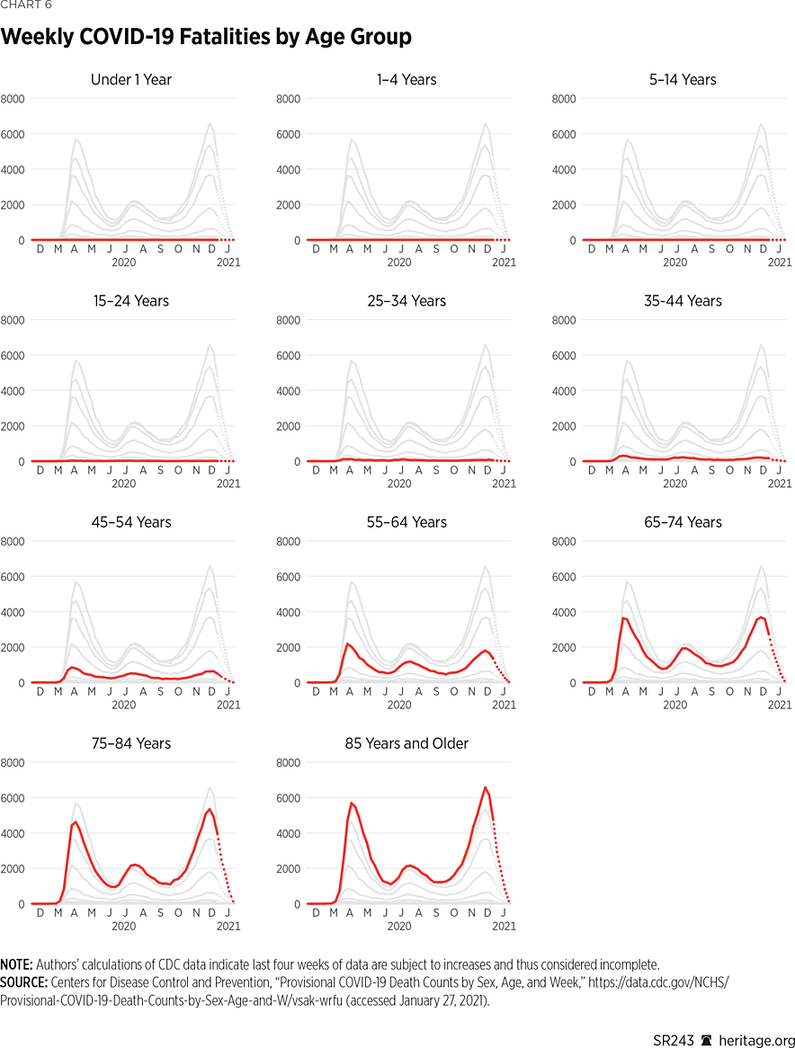
As Charts 5 and 6 demonstrate, the country also experienced new peaks in hospitalizations and fatalities in December. Numbers of fatalities across most age groups rose significantly in December, after a relatively mild second wave over the summer. Both charts make it apparent how much more dangerous COVID-19 has generally been for those ages 55 years and older. The following statistics, based on data provided by the Centers for Disease Control and Prevention, breaks down COVID-19 deaths by age as of January 27, 2021.
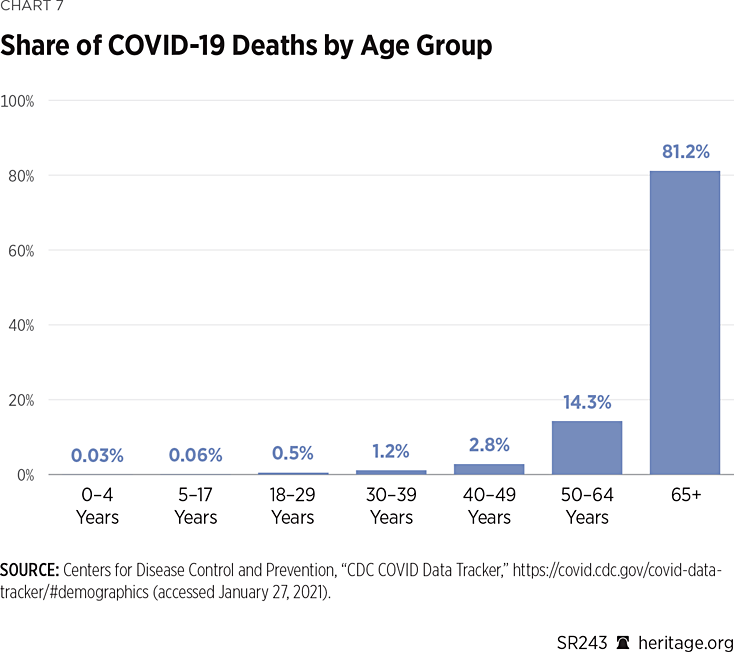
As Chart 7 illustrates, about 95 percent of COVID-19 deaths have been amongst people over the age of 50—signifying the COVID-19 death toll is heavily skewed towards the elderly. In fact, COVID-19 is just one of many respiratory infections that have been shown to be disproportionately dangerous to the elderly, as well as those with chronic conditions.REF This fact is particularly problematic in the United States, given that large segments of the population suffer from pre-existing conditions such as diabetes and obesity.REF
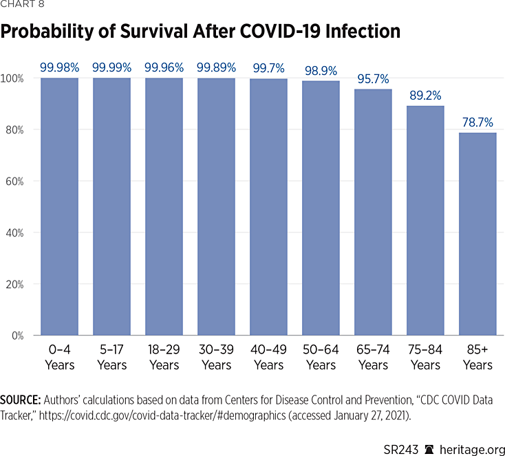
These statistics, however, only focus on those that have died from COVID-19 and exclude recovered cases. A challenging aspect of this type of analysis is that true infection rates are still unclear as there are many unconfirmed, particularly asymptomatic, cases that are not adequately represented in state and nationwide data.REF Using confirmed case data from the CDC, Heritage analysts computed the probabilities of survival by age upon contracting the disease.REF
As expected, the probability of survival is lower for the elderly than for younger age groups. However, these calculations also indicate that all age groups have a strong ability to fight COVID-19, as the probability of survival is notably greater than that of death across all age groups.REF In fact, all age groups under 65 have had a probability of survival upon contracting COVID-19 above 98 percent. Even among the two most vulnerable age groups in Chart 8 (ages 85 and up and ages 75–84) the chances of survival are over 75 percent and 85 percent, respectively. Thus, most people, including the elderly, also recover from COVID-19, and advances in medical treatments have significantly improved their ability do so.REF These estimates, however, are also based on confirmed cases and exclude unconfirmed cases. Infection fatality ratios, which include these unconfirmed cases (and thus incorporate more recoveries in the calculation), suggest even higher survival rates.REF
Regardless, an overwhelming fraction of the mortality of COVID-19 deaths have been confined to older age groups. Furthermore, data compiled by the COVID Tracking Project also demonstrates that over 36 percent of the COVID-19 deaths have been among long-term care facility patients alone.REF Chart 9 shows a comparison of the percentage or nursing home COVID-19 fatalities to overall COVID-19 fatalities in each state based on data provided by the Centers for Medicare and Medicaid Services.
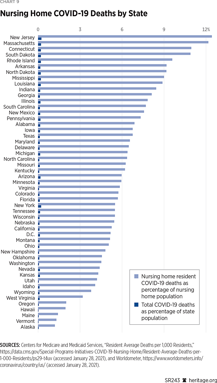
These data show that the percentage of COVID-19 deaths in nursing homes were significantly higher—over 50 times higher on average—than the general population’s mortality rate. This discrepancy illustrates that residents in nursing homes are particularly vulnerable and thus would have benefitted significantly from better protections during the course of the year.
This analysis demonstrates that COVID-19 has disproportionately impacted the elderly throughout the U.S. The following section examines the spread of COVID-19 on a geographic basis, analyzing how the disease has impacted different regions of the country.
Geographic Analysis of COVID-19
All 50 states have fundamentally different characteristics, including economies, population density, ethnic and age composition, and entering/exiting traffic, among others. As a result, some areas of the country are more prone to having higher levels of disease proliferation than others.REF It is therefore worthwhile to examine COVID-19 prevalence on a county-by-county basis both in terms of the actual number of cases, as well as a percentage of the country’s population. We do so in this section.
Figure 1 depicts monthly new COVID-19 infections across the country, from March 2020 through January 2021.REF As these charts illustrate, the northeastern area of the country had the greatest number of infections early in the pandemic. By the summer, however, the Northeast was no longer the nation’s hot spot for new cases. By then, Southern California, Arizona, and Florida had the country’s highest numbers of new infections. Other areas of the country, such as some localities in Michigan, Wisconsin, and Texas saw several thousand new monthly cases of COVID-19 from June through October 2020. In November, however, these areas, as well as Southern California, Florida, the Northeast, and a number of other pockets throughout the country became hotspots. These charts are consistent with findings in prior Heritage Foundation research; high levels of infections in the U.S. have been localized in different areas of the country during different times of the pandemic.REF
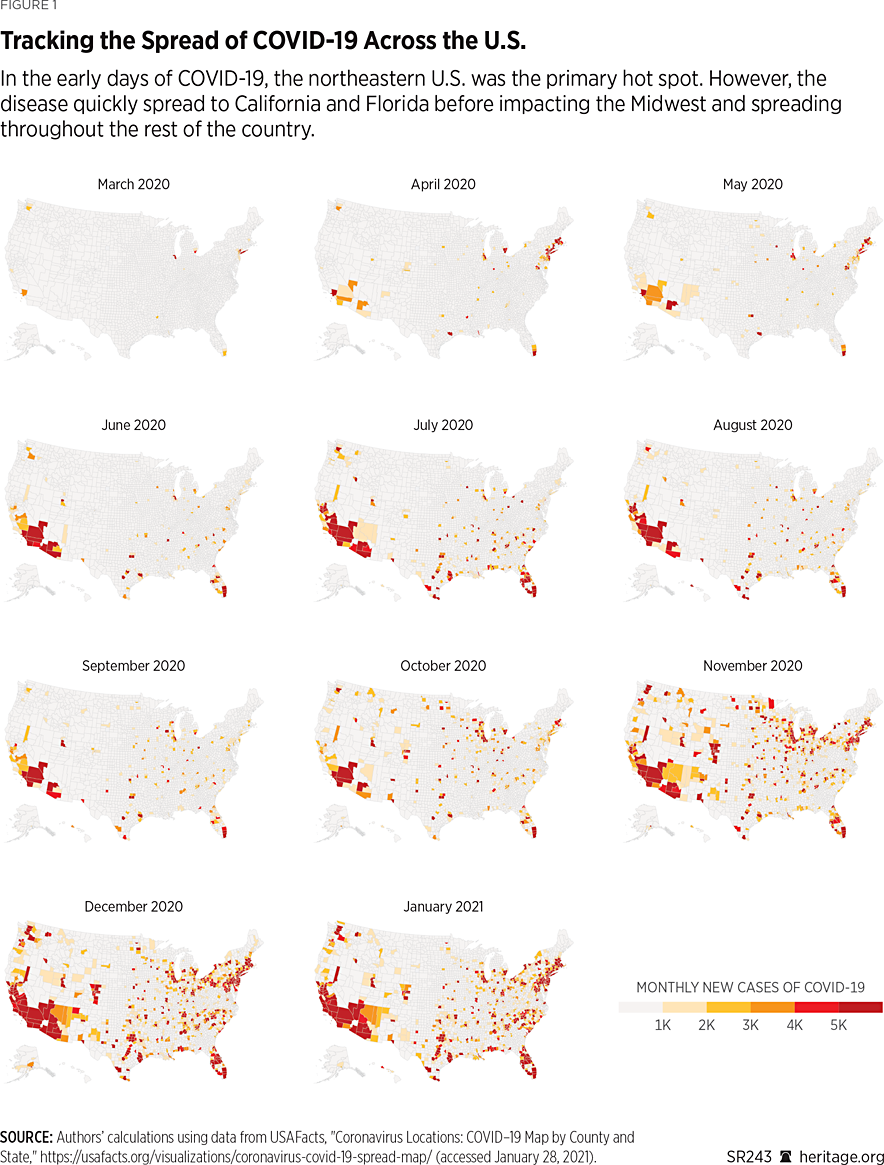
However, in recent months, the number of new cases has been more geographically dispersed among the population than during the earliest stages of the pandemic.REF For instance, from October 1 to November 12, half of the new cases spread among 182 counties in 42 states, where 49.4 percent of the U.S. population resides (roughly equal to the share of new cases).REF Still, despite California’s relatively strict lockdown rules throughout the year, relatively high growth in new cases continued to emerge at the end of summer through the winter.REF Governor Gavin Newsom (D–CA), nonetheless, maintained his strategy, announcing stay-at-home orders in December for certain areas of the state, with the goal of mitigating recent case growth and hospitalizations. In the subsequent section, we more closely examine trends in mobility and the efficacy of lockdown policies during COVID-19’s course in 2020.REF
Responses to COVID-19
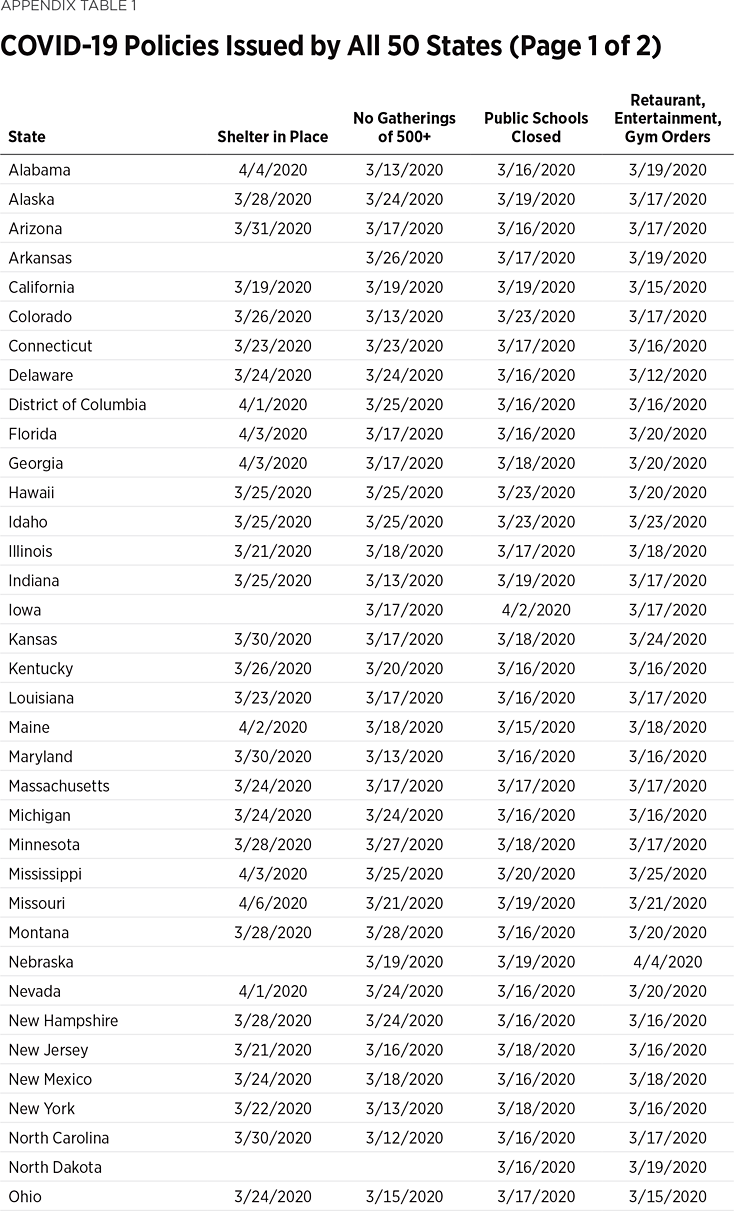
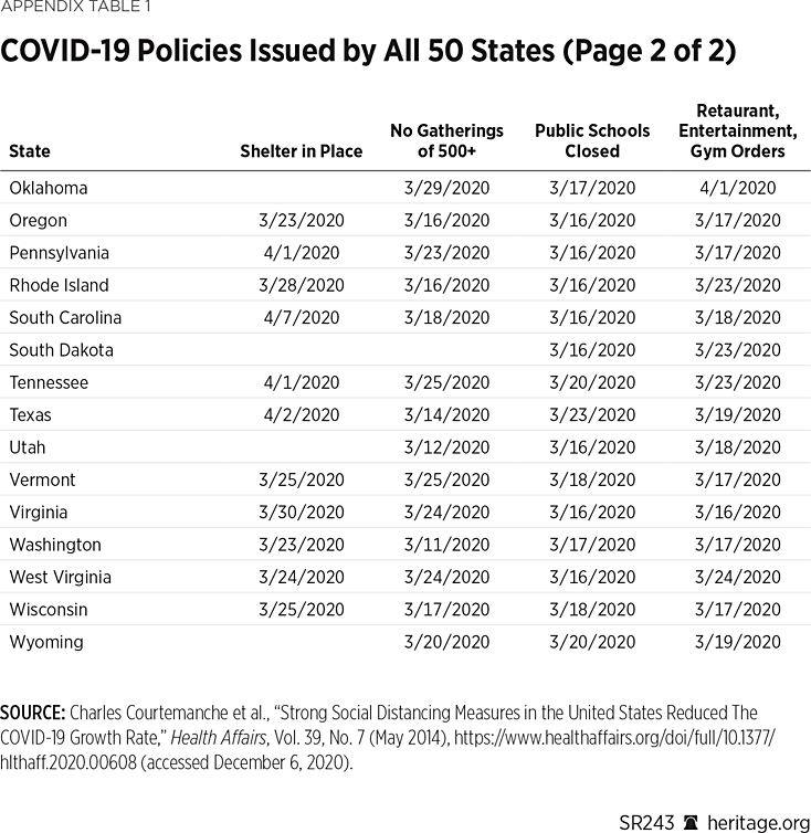
Once COVID-19 was declared a pandemic in the spring, significant efforts were taken by policymakers, as well as the general public, to limit the spread of the disease. In particular, 43 states (including the District of Columbia) imposed shelter-in-place orders and many Americans, either as a result of these orders or of their own volition, decided to stay home more frequently, frequent bars and restaurants less often, and work from home if possible.REF Exact dates of shelter-in-place orders are presented in Appendix Table 1.
Mobility Indices. Based on cellphone data, Google provides mobility indices aggregated across counties and states based on changes in people’s habits regarding certain categories that Google deems to be useful for understanding: (1) levels of social distancing; and (2) access to essential services. These categories include staying in one’s residence, visits to workplaces, visits to grocery stores/pharmacies, and visits to retail stores, among others.REF Estimates are provided on a daily basis with respect to a baseline value from earlier in the year.REF Specifically, each day’s baseline represents the median value for the corresponding day of the week during the five-week period from January 3, 2020, through February 6, 2020, for each particular category. For a particular state and category (residence, workplace, grocery stores/pharmacies, and retail store visits), each mobility index in the data set on a particular day represents the percentage change in mobility with respect to this baseline.
In this section, we present a series of data visualizations of the Google mobility data in states that issued shelter-in-place orders and states that did not. In addition, we analyze the Google mobility data using changepoint analysis, a statistical technique that can identify when the most significant changes in a time series of data have occurred. This technique uses the method of maximum likelihood to assess the entire time series and identify at the point at which the time series experiences the greatest change. Full details of the methodology are described in the appendix.
We discuss our changepoint analysis of the Google mobility data through May 31, 2020, which provides a sense of how people adapted to the pandemic during its onset the first several months of 2020. We also provide a variety of visualizations of the data comparing states that issued shelter-in-place orders to states that did not. Overall, this analysis helps provide a sense of the general public’s overall response to COVID-19, as well as overall compliance with associated lockdowns.
Residence Mobility. Charts 10-13 present Google mobility indices for staying at home, as well as visits to grocery stores, pharmacies, retail stores, and workplaces, averaged across the states that issued shelter-in-place orders and the states that did not between February 15, 2020, and January 22, 2021.REF Chart 10 offers some insights into people’s propensity to stay home during this time period.
As Chart 10 shows, states that issued shelter-in-place orders exhibited a slightly higher prevalence of people staying at home than states that did not issue such orders. For example, during the months of March, April, and May, the residency mobility index averaged 7.8 percent, 17.7 percent, and 12.7 percent, respectively, compared to January’s baseline activity. For states that did not issue such orders, on the other hand, the mobility index averaged 6.3 percent, 14.2 percent, and 9.2 percent for March–May, respectively, with respect to January’s baseline.
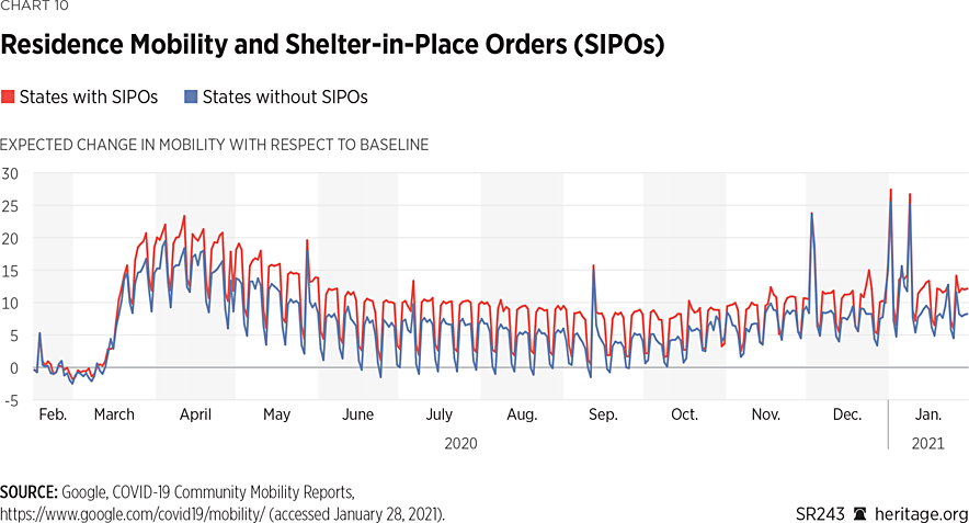
Since the summer, people gradually began to shelter in place less frequently and have trended toward baseline activity with respect to January’s baseline. This reversion toward baseline activity may have contributed to the recent spikes in cases presented earlier in Chart 10. For the most part, however, people both in states that have issued shelter-in-place orders, as well as those that have not, have still stayed at home at levels higher than baseline levels in January 2020 before COVID-19 was declared a pandemic on March 16. Specifically, average baseline residential activity in January 2021 averaged 11.6 percent in states that issued shelter-in-place orders and 8.8 percent in states that did not issue such orders (compared to baseline activity), each 11.3 percent and 8.9 percent higher than the average value of this index between February 15, 2020, and March 15, 2020—before COVID-19 had been declared a pandemic.
Our changepoint analysis indicates that, through May 2020, the overall trend in residence mobility for states issuing shelter-in-place orders experienced its largest change on March 16, 2020. The overall trend in residence mobility for states without shelter-in-place orders, however, experienced its largest change one day earlier, on March 15, 2020. Both of these changepoints are statistically significant (significance level of 0.05, p-value <0.01). These results indicate that, although states that issued shelter-in-place orders did seem to have people staying home more frequently than states that did not issue such orders, states belonging to either category exhibited a significant change in overall behavior at around the same time. In fact, the earliest state-wide shelter-in-place order occurred in California on March 19, 2020, showing that many people changed their behavior before the shelter-in-place orders had been instituted.REF
Grocery Stores and Pharmacies. Chart 11 depicts changes in visits to grocery stores and pharmacies, averaged across states that issued shelter-in-place orders and states that did not. As Chart 11 indicates, the pandemic initially decreased grocery store activity in states that issued shelter-in-place orders as well as states that did not, although this effect was much more pronounced in states that issued shelter-in-place orders. Specifically, during April, May, and June of 2020, the grocery/mobility index averaged 1.4 percent, –14.7 percent, and –3.0 percent, respectively, for states that issued stay-home orders. For states that did not issue such orders, on the other hand, the mobility index averaged 7.5 percent, –5.4 percent, and 8.4 percent March–May.
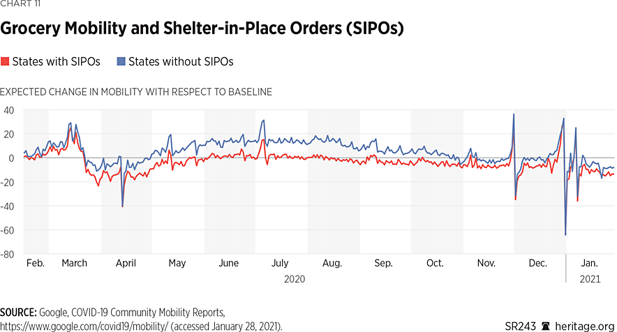
Both states that issued such orders and states that did not showed a spike in grocery store and pharmacy visits around Independence Day, Thanksgiving weekend, Christmas Day, and New Year’s Eve. During the fall, visits from both types of states have gradually returned close to baseline levels of activity in January, although activity has been trending downward since August. Our changepoint analysis indicates that before May 31, both states that issued shelter-in-place orders and states that did not had their most conspicuous change in overall grocery/pharmacy mobility on March 20, 2020.
The initial and recent decrease appears in the increased use of online grocery shopping. In fact, online grocery retailers such as Instacart, Peapod, and Amazon Prime saw a significant surge in demand, with which they had challenges keeping up.REF During the summer, however, grocery store activity resumed closer to baseline levels, and downward trends now may be due to concerns about the fall wave of cases.
Workplace. Chart 12 presents changes in workplace mobility averaged across states that issued shelter-in-place orders and states that did not. Once COVID-19 became a serious concern in the spring, protecting employees’ health became paramount to organizations across the country, and nearly half of businesses permitted workers to work remotely.REF Chart 12 depicts changes in workplace mobility over time. Our changepoint analysis indicates that amongst states that had issued shelter-in-place orders, the most conspicuous change through May 31 occurred on March 16. For states that did not issue such orders, this change occurred on March 15. Once again, as California was the first state to institute shelter-in-place orders on March 19, these changes occurred before such orders were issued.
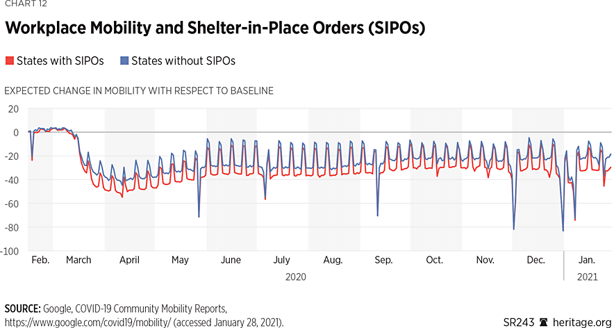
As Chart 12 illustrates, workplace mobility declined significantly in April in both shelter-in-place states and non-shelter-in-place states, with working from home being slightly more prevalent in the states that had issued shelter-in-place orders. Specifically, during the months of March, April, and May, the states that had issued shelter-in-place orders had a mobility index of –18.9 percent, –45.8 percent, and –36.4 percent with respect to January’s baseline, respectively, while the states that had not issued shelter-in-place orders noticed a mobility index of –14.2 percent, –36.6 percent, and –28.5 percent, respectively. Since the summer, workplace mobility has fluctuated in very similar manners amongst states that issued shelter-in-place orders as well as in states that did not, and has trended toward baseline activity, although it has not achieved original baseline levels.
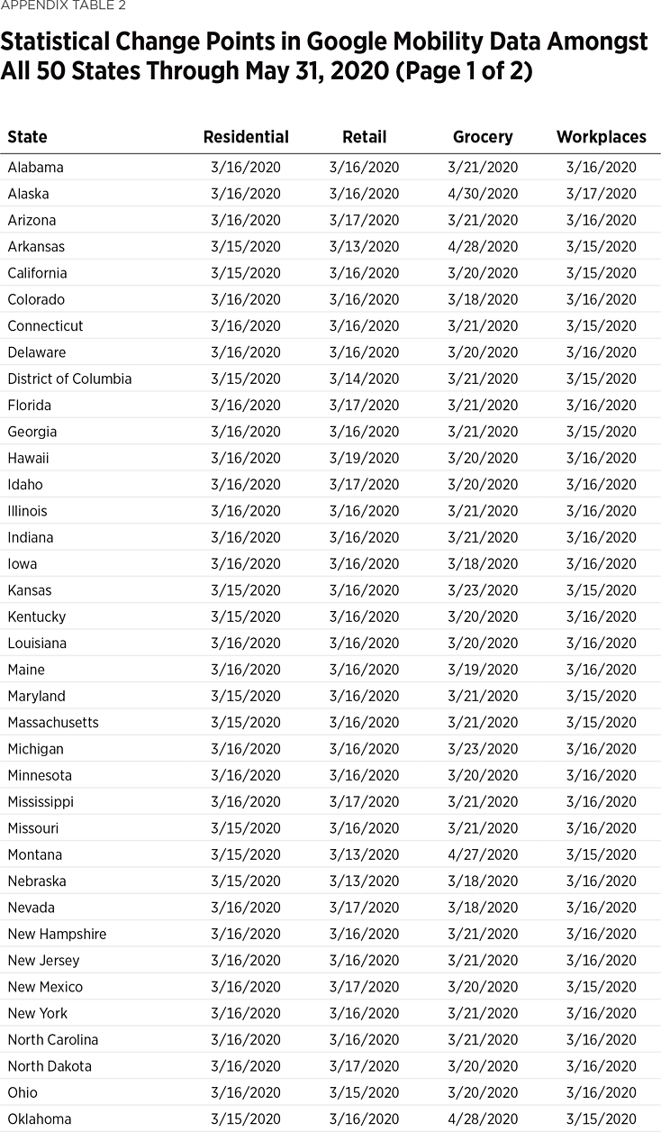
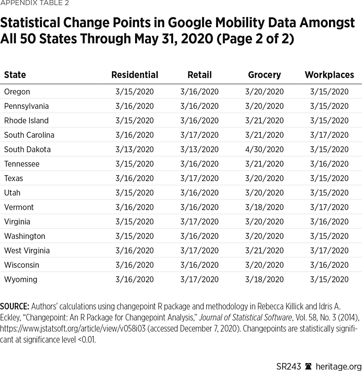
Retail Activity. Finally, Chart 13 provides a visualization of Google mobility data on visits to retail stores. As a result of the shelter-in-place orders, as well as people’s general hesitance to leave their homes out of safety concerns, many retailers closed their doors in the spring.REF Our changepoint analysis indicates that both states that issued shelter-in-place orders and states that that did not (as of May 31) experienced the greatest change in retail mobility on March 16, 2020. As Appendix Table 2 illustrates, only 12 states had issued prohibitions on restaurants, gyms, and entertainment venues on or before this date. These behavioral changes were thus mostly a result of people’s own volition.
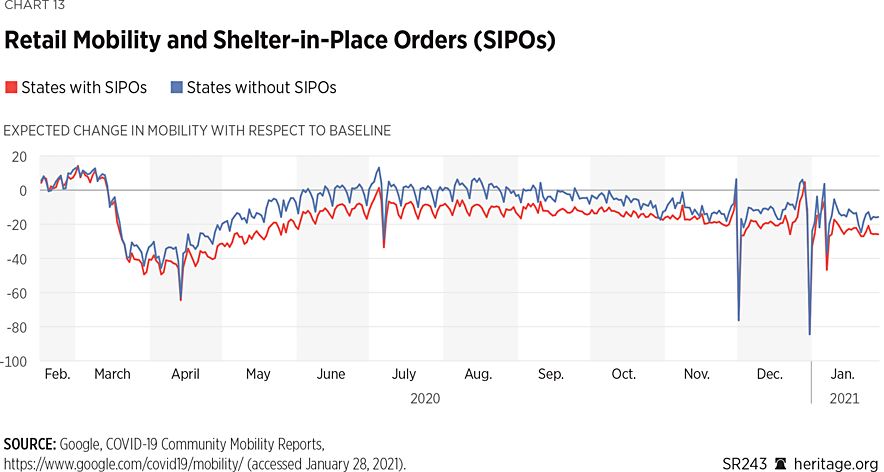
Furthermore, as Chart 13 illustrates, retail mobility declined significantly in April in both shelter-in-place states as well as non-shelter-in-place states with the decline in retail mobility being slightly more prevalent in the states that had issued shelter-in-place orders. Specifically, during the months of March, April, and May, the states that had issued shelter-in-place orders noticed a mobility index of –15.7 percent, –40.7 percent, and –24.7 percent, respectively, while the states that had not issued shelter-in-place orders noticed a mobility index of –12.4 percent, –32.4 percent, and –12.1 percent, respectively.
As with the other mobility indices, the trend of retail mobility consists of a tremendous drop before April, followed by a reversion to (without actually achieving) baseline activity over the course of the year. This trend back toward baseline activity may have contributed to the recent fall wave presented in Chart 13. However, retail activity is still not at levels it was before the pandemic had begun. Specifically, in January 2021 retail activity was –24.8 percent in states that issued shelter-in-place orders and –16.0 percent in states that did not (with respect to baseline activity), a –20 percent to –30 percentage point drop compared to average activity between February 15, 2020, and March 15, 2020.
Altogether, the Google mobility data suggests a number of important insights.
- The country exhibited a notable change in behavior because of the pandemic.
- States that issued shelter-in-place orders did track slightly higher behavioral changes in activity (staying at home, avoiding areas with other people, etc.) than states that did not.REF
- These behavioral changes, such as staying at home more frequently, frequenting retail stores less often, and working from home, in many cases became more prevalent before shelter-in-place orders had occurred.
- People gradually began reverting back to baseline activity during the past few months, which may have contributed to the recent fall wave. However, residence mobility data illustrates that people are beginning to stay home more frequently once again, likely due to concerns about increasing COVID-19-related cases and deaths.
In the next section, we examine the impact of these changes as well as government policies on case growth and the mortality of COVID-19.
The Impact of Policies and Behavioral Changes to COVID-19
As discussed in the previous section, 43 states (as well as the District of Columbia) implemented shelter-in-place orders to avert the spread of COVID-19. Different states instituted shelter-in-place orders at different times, and all states issued prohibitions on gatherings, restaurants, and school closures.REF Dates of implementation of these types of policies are included in Appendix Table 1.
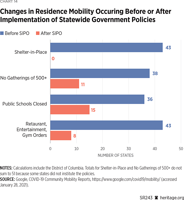
However, as discussed in the previous section, the Google mobility data illustrates that people dramatically changed their behavior early on in the pandemic, even before many of the orders were issued. We computed changepoints on a state-by-state basis for all 50 states (and the District of Columbia) for the residential mobility data.REF All changepoints are statistically significant (p-value <0.01). Our results are in Appendix Table 2 and summarized in Chart 14.
A few points stand out:
- All states experienced a change in residence mobility around March 15. The complete list of dates is contained in Appendix Table 2.
- Amongst all 43 states (including the District of Columbia) that implemented shelter-in-place orders, this change occurred before the orders were implemented.
- Amongst all 48 states (including the District of Columbia) that prohibited gatherings exceeding 500 people, 38 states experienced a changepoint in residence mobility before the policy had been instituted.
- Thirty-six out of 50 states (including District of Columbia) experienced a change in residence mobility preceding closures to public schools.
- Thirty-eight out of 50 states (including District of Columbia) experienced a change in residence mobility preceding closures of restaurants, entertainment venues, and gyms.
Survival Analysis. These results illustrate an important fact: Behavioral changes in response to COVID-19 preceded government policy changes in most states. It is also worthwhile to examine the efficacy of both these behavioral changes as well as the changes in response to policies intended to curb the impact of COVID-19. To do so, we drew upon a well-known statistical methodology known as survival analysis, used to assess the impact of factors influencing the duration of time before a particular event occurs.
Survival analysis has been used in many fields, such as the assessment of factors influencing cancer survival, reliability analysis in engineering, customer retention in marketing, default risk in finance, and recidivism in criminology.REF To understand the effect of various directives by state governors of COVID-19, we developed a survival model to assess the impact of policies and behavioral changes on case growth and mortality across all 50 states and the District of Columbia. The results of our analysis enable us to understand the degree to which these factors ultimately impacted the time to reach specific per capita levels of case growth and mortality.
Specifically, the dependent variables in our analysis were the time for a state to exceed a particular threshold (maximum case growth, per capita deaths for a variety of different per capita thresholds) through August 2020.REF These thresholds were assumed to follow a Weibull distribution, a workhorse model in survival analysis.REF Our independent variables, in terms of government policies, were the number of days from the state’s first confirmed COVID-19 case to the issuance of shelter-in-place orders and the prohibition of gatherings of more than 500 individuals (as described in the appendix). In addition, we also included as an independent variable the number of days from the state’s first confirmed COVID-19 case to the behavioral change in residence mobility which, as discussed earlier, was calculated in terms of the state’s changepoint through May 31, 2020.REF The changepoints that we estimated for each state are listed in Appendix Table 2. Across the states examined (as well as the District of Columbia), the average time from a state’s first case to its imposition of shelter-in-place orders (if such policies were instituted) was 25.02 days (standard deviation 13.43 days). The average time from a state’s first case to the imposition of prohibitions on gatherings above 500 people (if one was instituted) was 16.10 days (standard deviation 12.64 days). Finally, the average time from a state’s first case to its changepoint in residence mobility was 11.88 days (standard deviation 13.03 days).REF
As discussed earlier in this report, all 50 states are fundamentally different in nature. For example, there is no a priori reason to believe that New York residents will respond to COVID-19-related policies in the same exact manner as people in Texas. As a result, it is important to incorporate state-level heterogeneity in any statewide policy modeling.REF We did so by constructing a hierarchical Bayesian survival model in which state-level coefficients are drawn from a lower-dimensional prior distribution. Specifically, we allowed our regression coefficients to follow a multivariate normal prior with non-zero correlations alongside informative hyperprior distributions. This technique enables us to allow each state to have a unique response to measures instituted while providing pooled estimates across all states that quantify the overall effect of these responses. Full details of our regression model are discussed in the appendix.
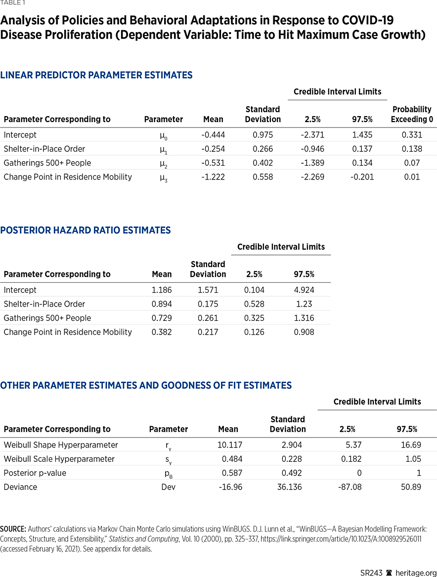
In our first set of simulations, we examined the impact of shelter-in-place orders and change in behavior on the time for a state to achieve its maximum case growth rate. Our results from our estimation are presented in Table 1.REF
Goodness-of-fit tests, via posterior p-values, indicates that the model fits the data quite well, and it is thus reasonable to draw inferences from the coefficients. Negative coefficients for the linear predictor function demonstrate that the associated policies, as well as the actions taken by individuals, slowed the time to achieve maximum case growth. In particular, our model’s results indicate that the more quickly a state issued shelter-in-place orders (–0.254, and probability exceeding zero 0.138) and restrictions on gatherings above 500 individuals (posterior mean –0.531, and probability exceeding zero 0.070), the longer it took them to achieve maximum case growth. These measures therefore had some contributions in flattening the state’s case curve. The associated marginal posterior hazard ratios, however, have upper 95 percent credible intervals limits exceeding one. These results indicate that the measures had limited efficacy in quelling case growth.
However, changes in each state’s aggregate residence mobility index, as indicated from the coefficient associated with the incidence of the state’s first case to its changepoint, is larger both in terms of magnitude and negative density (posterior mean –1.222, probability exceeding zero 0.01). The associated posterior hazard ratio of this coefficient has posterior mean 0.382 and 95 percent credible interval [0.126, 0.908]. Unlike the other variables examined, the posterior intervals suggest that these behavioral changes are the only effect that is significant. These results indicate that the more quickly states experience a behavioral change in residence mobility, the longer they are able to delay achieving maximum case growth in the time period examined.
Altogether, our results suggest that these behavioral changes quelled case growth more than government policies did. This finding is not surprising because, as discussed in the prior section, as well as Appendix Table 2, people began changing their behavior before shelter-in-place orders were issued, suggesting that they were seriously concerned about the disease before the implementation of government shutdown policies.
In another series of simulations, we looked at the impact of state-based policies on the time to reach a particular per capita mortality rate. Tables 2–4 depict our results examining the impact of the time from each state’s first case to implementing shelter-in-place orders, prohibitions on gatherings exceeding 500 people, and changes in behavior as elicited by changepoints in the Google residence mobility data to the onset of the state’s first confirmed COVID-19 case on the time to reach 2, 10, and 20 deaths per million individuals.
Once again, our posterior p-values indicate that the Weibull survival model fits our dataset well, and thus we can justifiably draw statistical inferences from our coefficient estimates. The linear predictor coefficients corresponding to the policies state governors instituted, along with behavioral changes individuals made to shelter in place more frequently, all have negative posterior means, suggesting that these measures collectively delayed the time to achieve the specified threshold of per capita deaths. The associated posterior hazard ratios are all less than one. According to our posterior intervals, however, the coefficients associated with the shelter-in-place orders are significant for all three mortality-related simulations. In particular, for the simulation involving the time to reach two deaths per million, the posterior hazard ratio associated with time from the first case to the imposition of shelter-in-place orders was 0.620, with a (0.409,0.836) 95 percent credible interval. For the simulation involving the time to reach 10 deaths per million, the posterior hazard ratio was 0.638 with a (0.438,0.870) 95 percent credible interval. Last, for the simulation involving the time to reach 20 deaths per million, the posterior hazard ratio was 0.629 with a (0.408, 0.873) 95 percent credible interval. These three estimates are statistically the same up to their associated 95 percent credible intervals.
Additionally, two of the three simulation results also illustrate that prohibitions on gatherings of more than 500 people also has an effect on quelling deaths. As Tables 2–4 illustrate, as was the case with the coefficients corresponding to the shelter in place orders, the linear predictor coefficients are also negative. Additionally, for the simulation involving the time to reach two deaths per million, the posterior hazard ratio associated with time from the first case to the imposition of prohibition of gatherings above 500 was 0.526 with a (0.235,0.892) 95 percent credible interval. For the simulation involving the time to reach 10 deaths per million, the posterior hazard ratio was 0.541 with a (0.247,0.941) 95 percent credible interval. However, for the simulation involving the time to reach 20 deaths per million, the posterior hazard ratio was 0.598 with a (0.203, 1.325) 95 percent credible interval (and was thus not significant). These coefficients thus increase in magnitude with respect to the thresholds examined.
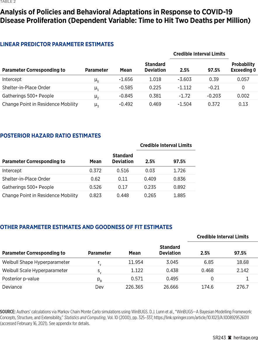
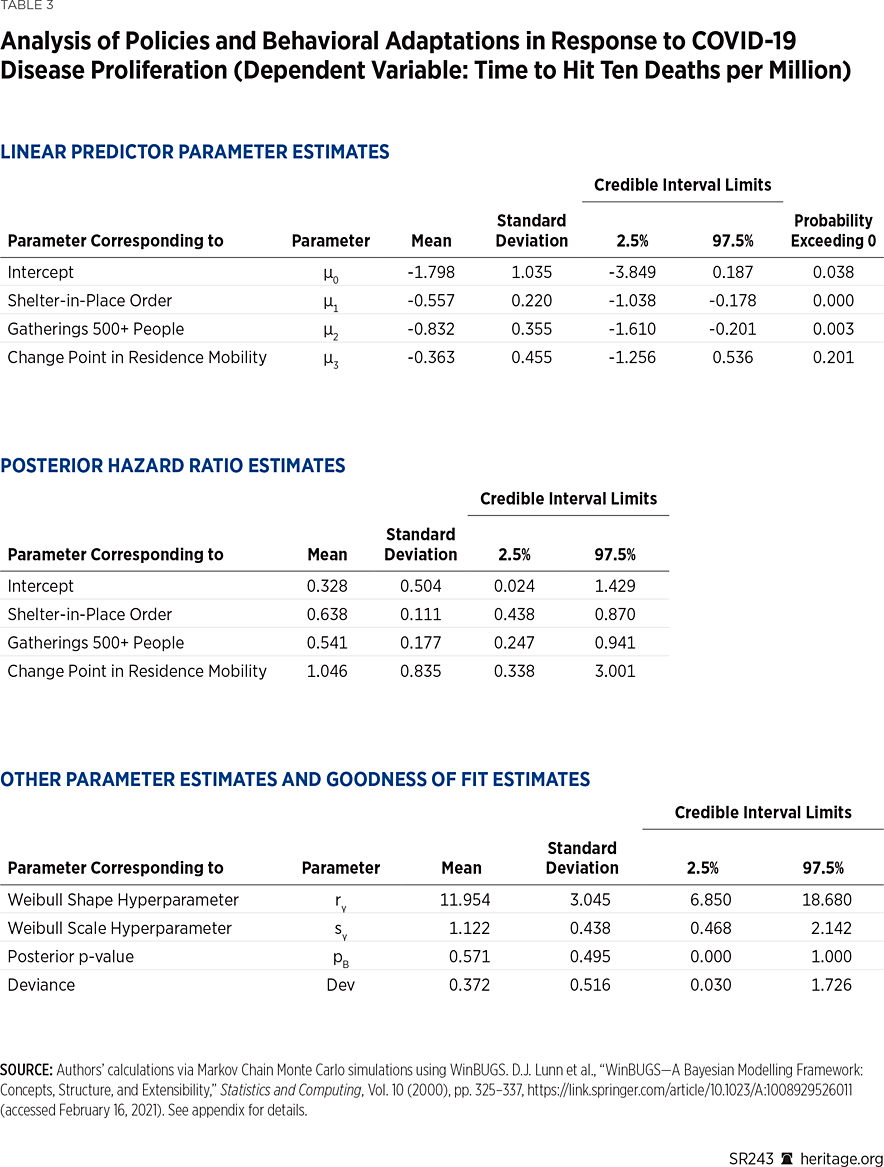
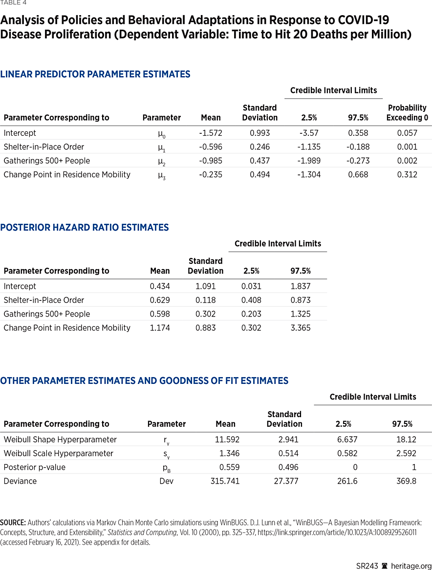
However, unlike the regression involving case growth as the dependent variable, the coefficients pertaining to the changepoints are smaller in magnitude than coefficients pertaining to the shelter-in-place orders and prohibitions on gatherings exceeding 500 people. In fact, the changepoint coefficient increases for each simulation and has non-trivial positive posterior density. With the dependent variable being the time to reach two deaths per capita, the posterior mean of the linear predictor coefficient is –0.492 (probability exceeding zero 0.13); with the dependent variable being the time to reach 10 deaths per capita the posterior mean is –0.363, with the probability exceeding zero being 0.201; and with the dependent variable being the time to reach 20 deaths per capita the posterior mean is –0.235 with probability exceeding zero equaling 0.312. The analysis also indicates that the posterior hazard ratios pertaining to the changepoint are not below one within the 95 percent credible interval. These results suggest that behavioral changes were not as effective for quelling mortality as they were for quelling case growth. Shelter-in-place orders and prohibitions on large gatherings, on the other hand, elicited a stronger effect on the time to reach the mortality thresholds the authors examined.
This difference is likely due to the fact that, as discussed earlier in this report, mortality is most heavily pronounced amongst the elderly and those with chronic conditions, with over 36 percent of COVID-19 deaths occurring in nursing homes.REF As discussed in Chart 8 earlier, however, all age groups under 65 have had a probability of survival upon contracting COVID-19 above 98 percent. As these probabilities decline for older age groups, proper measures aimed at protecting these people (beyond just staying at home) could have significantly increased their survival trends toward the levels of younger cohorts.
Moreover, in all of our simulations, the marginal posterior estimates of the hyperparameters determining the Weibull density’s scale parameters indicates that as time goes on, each state is more likely to achieve the specified per capita mortality threshold.REF Thus, in many regards, reaching the mortality threshold is somewhat policy invariant given enough time. Again, this result is likely due to the fact that the most vulnerable could have been much better protected throughout the pandemic, especially during early stages of the crisis.
Discussion
Our analysis demonstrates that the time from a state’s first case to voluntary changes in residence mobility, which occurred before the imposition of shelter-in-place orders in 43 states, indeed quelled the time to reach the maximum growth in per capita cases. On the other hand, our analysis also indicates that these behavioral changes were not significantly effective in quelling mortality, while government measures were. Specifically, our simulations find a negative effect of the time from a state’s first case to the imposition of shelter-in-place orders on the time to reach the specified per capita mortality thresholds. Our analysis also finds a slightly smaller negative effect on the time from a state’s first case to the imposition of prohibitions on gatherings above 500 people.REF
However, caution should be taken in interpreting the results pertaining to the impact of shelter-in-place orders on the time to reach the mortality thresholds examined. Most notably, the marginal posterior hazard ratio for the time from the first case to the prohibitions on gatherings above 500 people increased in magnitude between the simulations examining the time to reach two deaths per capita and the time to reach 10 deaths per capita, suggesting that the policy may have indeed delayed the time to reach this higher level of mortality. On the other hand, the analogous coefficient estimates for shelter-in-place orders across all three mortality simulations were statistically the same (up to the 95 percent credible interval), suggesting that shelter-in-place orders did not help stave off achieving higher per capita mortality thresholds (20 deaths per million) than they helped delay reaching lower levels (two deaths per million) levels.
Furthermore, as Chart 7 illustrates, over 80 percent of COVID-19 deaths occurred amongst individuals over the age of 65, and over 95 percent of deaths occurred amongst individuals over the age of 50. Additionally, deaths in younger-age cohorts have been heavily confined to those with pre-existing conditions.REF Thus, the effect of shelter-in-place orders on quelling mortality in Tables 2-4 is likely a manifestation of many of these higher risk people sheltering in place.
Moreover, shelter-in-place orders can also have negative unforeseen health-related consequences, including the capacity to cause patients to avoid visits to doctors’ offices and emergency rooms. In addition, these policies can result in people, including those with chronic illnesses, skipping routine medical appointments, not seeking routine procedures to diagnose advanced cancer, not pursuing cancer screening colonoscopies, postponing non-emergency cardiac catheterizations, being unable to seek routine care if they experience chronic pain, and suffering mental health effects, among others.REF In fact, drug overdose deaths, alcohol consumption, and suicidal ideation have also been noted to have increased in 2020 compared to prior years.REF Unfortunately, we are unable to include or control for these effects in our analysis, and their effects will only become more apparent in the coming years.
Additionally, as discussed earlier, 36 percent of COVID-19 deaths occurred in long-term care facilities. We were also unable to properly control for this occurrence in our analysis, as complete state- and county-level daily nursing-home mortality data from the beginning of the pandemic remains unavailable.
Thus, the use of blanket shelter-in-place orders during this pandemic is tantamount to killing a fly with a sledgehammer. Given how narrowly focused the mortality of COVID-19 has been, alternative and more targeted policies could have more effectively combatted the disease that would not have had unforeseen consequences such as those mentioned above. Previous Heritage Foundation research, for example, has suggested aggressive testing, a targeted approach toward protecting the most vulnerable, and the use of voluntary isolation centers would have been significantly more effective at preventing disease spread and mortality.REF
Policy Implications
Our analysis offers the following policy recommendations, from which lawmakers can apply to the remainder of this pandemic and learn from for the future.
Protect the Elderly and Most Vulnerable. As our analysis indicates, over 80 percent of COVID-19 deaths have occurred amongst individuals over the age of 65, and over 95 percent of COVID-19 deaths have occurred amongst individuals over the age of 50. Those with pre-existing conditions in younger age groups may also be prone to severe infection. However, as the statistics in this paper illustrate, younger age groups in general have had significantly lower levels of catastrophic illnesses. Early in the pandemic there was limited information about who was most vulnerable, but as Charts 7 and 8 show, although we have had that information for some time, the policies have not caught up sufficiently. Policies should have been geared toward protecting the most vulnerable. One-size-fits-all measures that fail to account for differences in age are unlikely to produce positive results—and may have significant negative health impacts.REF
Improve Data Collection on Nursing Homes. As discussed in this report, over 36 percent of COVID-19 deaths occurred in long-term care facilities. Chart 9 illustrates the level to which COVID-19 has disproportionately impacted nursing homes compared to overall populations. Sadly, throughout the pandemic, limited information has been available on nursing home deaths. The Centers for Medicare and Medicaid Services should release county-level COVID-19 statistics that include nursing home cases and deaths—both for residents and staff—and should consider doing so for other life-threatening illnesses as well.
Hot Spots and Problems Are Localized. As Map 1 shows, different areas of the country are more prone to developing higher rates of infection than others. As a result, during a crisis of this nature, state and local lawmakers should be given the flexibility to deal with events as they unfold. Our regression analysis in the previous section has indicated that policies and voluntary measures taken by individuals have all helped quell case growth. However, as the analysis also indicates, behavioral changes did not materially impact the death toll and, in terms of the policies instituted, were somewhat policy-invariant given enough time. Policies aimed at protecting the elderly, particularly in nursing homes, would have been much more helpful.
Conclusion
COVID-19 has plagued the country and the world unlike any malady since the Spanish flu of 1918.REF This research provides lawmakers with a statistical analysis of the virus and proposed policies to mitigate its impact. As we continue to fight this dangerous disease in the coming months, this study provides useful analysis and insights for lawmakers. In particular, the evidence shows that people changed their behavior before many government policies were implemented—but that more specific policies geared toward protecting the elderly, especially those in nursing homes, could have been much more effective at saving lives. Our empirical approach also provides a useful framework for analysis if a similar public health emergency arises in the future.
Appendix
Survival Model
We utilized a hierarchical Bayesian Weibull hazard model for states iϵ{1,…,51} states (including Washington, DC) and covariates pϵ{0,…,3}:
$$t_i∼Weibull(x_{i,0} x_{i,1},x_{i,2},x_{i,3}; α_{i,} γ_i ),$$
where ti is the dependent variable of interest, which in this paper is either the number of days from the first confirmed COVID-19 case to the maximum in case growth rate (Simulation 1)REF or the number of days from the state’s first confirmed COIVD-19 case to the time to reach a specified per capita number of deaths (Simulations 2–4). Our explanatory variables xi,1, xi,2, and xi,3 are specified as follows: For state i, xi,1 was the time from the state’s first confirmed COVID-19 cases to the state’s shelter-in-place order,REF xi,2 was the time from the state’s first confirmed COVID-19 cases to the state’s prohibition on gatherings exceeding 500 people, and xi,3 was the time from the state’s first confirmed COVID-19 cases to the time when public schools were closed. The probability density function we assumed for the Weibull distribution is parameterized as followsREF:
$$f(t;α_i, γ_i )=γ_i α_i t^{γ_i-1} exp(-α_i t^{γ_i } )$$
where α=(α1,,…αI ) and γ=(γ1,…γI,). This density function provides us with the following likelihood specification:
$$L(α,γ;t_1,..t_I )=\Pi^I_{i=1}f(t_i;α_{i,} γ_i )^{1-\delta_i} S(t_i;α_{i,} γ_i )^{\delta_i}$$REF
$$S(t;α_{i,} γ_i)=1- \int^t_0f(t^{'};α_{i,} γ_i )dt^{'}$$
and δi=1 if the dependent variable of interest is right censored (when a state does not achieve the desired threshold over the time horizon examined) and δi=0 otherwise. The model is parameterized via the following linear link function and choice of prior distributions:
$$log(α_i )=\beta_{i,0}+\Sigma^P_{p=1}\beta_{i,p} x_{i,p}$$
$$(\beta_{i,0,…,}\beta_{i,P} )∼MVN(\mu_\beta,\Sigma)$$
$$μ_\beta∼MVN(\mu_\beta,\Sigma_\beta ) $$
$$Σ^-∼ Wishart(\Sigma_0,P)$$
$$γ_i∼\Gamma(r_γ,s_γ )$$
$$r_γ∼\Gamma(a,b)$$ $$s_γ∼\Gamma(c,d).$$REF
We computed the changepoint in staying at home using the Google residence mobility data discussed in the mobility analysis section.REF We did so on a state-by-state basis using standard techniques in time series analysis by estimating the maximum likelihood function across different choices of potential changepoints across the time series for both states that issued shelter-in-place orders and states that did not.
One can compute the hazard ratio from the above survival function:
$$h(t)=f(t;α_{i,} γ_i )/S(t;α_{i,} γ_i ).$$
As a result, it is easy to see that the associated hazard function of the Weibull distribution is h(t)=αi γi tγi-1. Coupling this hazard function with the above link function connecting αi to our linear predictors results in each state’s proportional hazard rate HR for a particular covariate xi,p being HR=eβi,p. We averaged these hazard rates across all 50 states and the District of Columbia to generate a single-pooled estimate for each coefficient.
We ran our simulations in WinBUGS for 300,000 iterations with 30,000 for burn in. For all simulations, the Geweke convergence diagnostic finds statistical insignificance between the early iterations from the sampler (post burn-in) compared to the later iterations amongst all posterior coefficients, illustrating that the Markov Chain Monte Carlo sampler achieved convergence and our posterior samples thus adequately characterizes the posterior distribution.REF Goodness-of-fit tests were conducted to assess the efficacy of the survival model using chi-squared test statistics to estimate posterior p-values as discussed in Ntzoufras (2009) and Gelman et al. (2014).REF
Changepoint Detection
We conducted a changepoint analysis using Google’s residence mobility data for all 50 states (and the District of Columbia). For tϵ{1,2,...,T} given a time series yt with probability distribution p(yt│ϑ), under the null hypothesis of the non-existence of a changepoint, we assume the distribution of our time series is p(y1:T│ϑ) where ϑ is the maximum likelihood estimate of the distribution. The maximum log likelihood of this distribution is thus ML0 (ϑ)=log(p(y1:T │ϑ)). Under the alternative hypothesis, we can consider a model with changepoint τ1ϵ{1,2,...,T-1} and thus maximum log likelihood ML(τ1;ϑ1,ϑ2) for a given τ1 as follows:
$$ML(τ_1;\vartheta_1,\vartheta_2)=log(p(y_{1:τ_1} |\vartheta_1))+log(p(y_{τ_1+1:T} |\vartheta_2)).$$
Using these two functions, we used the R package changepoint that constructs the following test-statistic:
$$\lambda=2(max┬(τ_1 )ML(τ_1;\vartheta_1,\vartheta_2 )-ML_0 (\vartheta)),$$
and compare this statistic to a critical threshold to determine the changepoint and associated p-values as discussed in Killick and Eckley (2014).REF
Kevin Dayaratna is Principal Statistician, Data Scientist, and Research Fellow in the Center for Data Analysis, of the Institute for Economic Freedom, at The Heritage Foundation. Andrew Vanderplas is Special Assistant and Research Associate in the Institute for Economic Freedom.


