Executive Summary
This paper tries to capture the effects of interventions by government-sponsored enterprises (GSEs) in the housing market by creating a hypothetical scenario in which one could see what would happen to housing starts without Fannie Mae and Freddie Mac. Housing starts are an especially important indicator of overall strength in the housing sector and are a contributor to economic growth. This study finds that shutting down Fannie and Freddie during the test period of 1980–2010 would have slightly affected housing starts at the national and regional levels. The analysis uses time series regression models with quarterly data across a 30-year period to examine the effects of changes in conventional mortgage interest rates on housing starts both at the national and regional levels. The study controls for economic fundamentals—including real gross domestic product, price-to-rent ratio, median home price, vacancy rate, Consumer Price Index, household assets, household debt, and family income—to measure the effects of changes in mortgage interest rates on housing starts. The results indicate:
- A higher conventional mortgage interest rate would have had a minor negative impact on housing starts both at the national and regional levels, all other things equal. Based on the assumption that Fannie Mae and Freddie Mac did not exist in 1980–2010, the econometric results of this study suggest housing starts would have been lower by a mere 0.05 percent at the national level over this period.
- The effects of the GSEs appeared to vary by region. Housing starts over this time period would have been lower in the Northeast and Midwest by 0.005 percent and by 0.01 percent in the West and South.
- The South and West seem to be more sensitive to changes in mortgage interest rates because, as discussed by many scholars, they are more land regulated and have higher population densities.
- In sum, the results indicate that fundamentals—such as real output, the price level, family income, the total value of household assets, the ratio of average housing prices to renting, and the level of household debt—are by far the most important factors shaping housing starts at both the national and regional levels. In contrast, the conventional mortgage interest rate plays a minor role in shaping housing starts.
- The implication of these results for policy is straightforward: once housing and financial markets recover from the recent turmoil, shutting down Fannie and Freddie would only slightly affect housing starts nationally, although the effect would vary slightly by region because of land regulations and higher population densities.
Abstract
This empirical study tries to identify the main determinants of housing starts by measuring the responsiveness of housing starts to the mortgage interest rate compared with economic fundamentals at the national and regional levels. If housing starts are not responsive to changes in the mortgage interest rate, then interventions by government-sponsored enterprises in the housing market that lower mortgage interest rates would not significantly affect housing starts. Econometric analysis of the supply side of the housing market suggests that economic fundamentals, not mortgage interest rates, drive housing starts. Therefore, shutting down Fannie Mae and Freddy Mac would likely have little effect on the housing starts.
Housing starts are an important element of residential investment, an important component of total economic output. Previous Heritage Foundation studies on the housing market addressed the demand side of the housing market.[1] Of course, the supply side of the market responds to demand, so the extent to which the government-sponsored enterprises (GSEs) Fannie Mae and Freddy Mac affect housing should be equally apparent on the supply side, as measured by housing starts.
Although prices would be expected to play an important role in shaping housing starts, this has frequently not been the case. For instance, as Charles G. Nathanson and Eric Zwick argue, over some periods, cities such as Las Vegas experienced enormous construction rates relative to other cities, while real home prices remained relatively constant. Then, as prices subsequently doubled between 2000 and 2006, housing starts remained high. Indeed, housing starts were high despite rising prices because prices matter during a downturn, but not during a boom.[2]
If housing starts are not responsive to price changes, then other factors may have contributed to regional differences. Indeed, many scholars assert that regulations played an important role in limiting the amount of the land available for residential housing. Edward Glaeser argues that restricting housing supply through regulations leads to greater volatility in housing prices.[3] He compared the Boston region with the Atlanta region, which issues about seven times as many permits as the Boston region, and found that housing prices in Boston were much higher and more volatile than housing prices in Atlanta. In addition, Atlanta did not share in the Boston Boom of 1980–1988 when prices doubled or suffer from Boston’s housing bust of 1988–1994 when prices lost 50 percent.[4]
In assessing the causes of the housing bubbles, many scholars have focused on the demand-side factors, such as low interest rates, zero down payments, and easy lending terms. However, as Randal O’Toole argues, the demand-side factors were more or less equal across all states, but a more severe bubble was observed in a few states.[5] O’Toole argues that land-use regulation was the most important factor in the housing bubble of 2006. He supports this argument by finding a strong correlation between growth management planning and housing bubbles.[6] Although the land regulations have played an enormous role in creating the bubble and its subsequent bust in some states, one cannot rule out the importance of other economic fundamentals in creating the conditions for boom-bust behavior in the housing market.
Both demand and supply factors may contribute to the story. Indeed, with supply constraints and regulations in place, bubbles can form with a small increase in demand. With an inelastic housing supply (vertical supply curve), a small increase in demand can lead to huge a increase in housing prices. In other words, land-use regulations and geographic land constraints can have important effects on housing booms and busts, but this is not the whole story. As seen in the more detailed econometric results, many other economic fundamentals affect housing starts.
Economists have not reached a consensus on the specification of housing supply models. In earlier studies, housing starts were a function of the level of price and construction costs.[7] but more recent studies link housing starts to changes in housing prices and costs.[8]
On the demand side, the Federal Reserve’s policy of maintaining extraordinarily low short-term interest rates, which contributed to lower mortgage interest rates in 2003 and thereafter, intensified the housing price boom, which occurred because of easy access to mortgage credit, among other factors. While the results reported in this paper show that high interest rates may not affect housing starts, it appears that low interest rates, in part, steered individuals to purchase new houses.
Housing starts jumped up by the end of 2003 and remained high until the bubble burst in early 2006. The rise in demand for real estate accelerated housing price inflation, which reached 10 percent in the fourth quarter of 2004 and remained over 10 percent for the two consecutive years.[9] With the rise in housing prices, delinquency and foreclosure rates started to fall. However, as short-term interest rates returned to their initial levels, demand fell sharply and housing prices dropped below their equilibrium levels, bringing down home equities to levels lower than their mortgages. Underpriced home values, along with hikes in delinquency and foreclosure rates, led to the bubble bursting and the meltdown in the housing market in 2007. In fact, both the demand and supply sides of the housing market contributed to the meltdown, which put millions of borrowers upside down with negative equities. The five states with highest percentages of negative equities in 2009 were Nevada (65 percent), Arizona (48 percent), Florida (45 percent), Michigan (37 percent), and California (35 percent).[10]
Currently 11 million people are underwater with an average negative equity of $70,000, which means a total loss of around $770 billion[11] Whether the boom-bust behavior is attributed to the demand side or the supply side of the market, policymakers should immediately shut down Fannie Mae and Freddie Mac completely and permanently.[12] Replacing the GSEs with private players would stabilize the housing market and save taxpayers billions of dollars. Replacing GSEs with private players should take place before the Administration presents another bailout plan and burdens taxpayers more.
This paper first reviews the literature on the determinants of housing starts. Next, it discusses a theoretical model based on the literature review. The data section reviews the list of variables, their summary statistics, and their resources. The stylized facts section analyzes some of the trends in housing starts at both the national and regional levels. The econometric section measures the responsiveness of housing starts at the national and regional levels to changes in mortgage interest rates, controlling for a series of economic fundamentals. Finally, the analysis ends with a conclusion and policy discussion.
Literature Review
Although the literature has well documented the importance of the housing market, the number of studies on housing starts is relatively limited. This section reviews the seminal studies on the main determinants of housing starts to uncover how shutting down Fannie and Freddie could affect housing starts.[13]
J. R. Kearl estimates housing starts as a function of income, price index, interest rates, and household characteristics such as family size. He finds that inflation has a negative distortive effect on housing starts and a housing supply elasticity of –0.39 to nominal interest rate.[14] In other words, a 1 percent increase in nominal interest rate is associated with a 0.39 percent decrease in housing starts.
Christopher Mayer and Tsuriel Somerville are among the few that estimate housing supply elasticities by Census Bureau region. Using data from 1975 to 1994, they model housing starts as a function of changes in housing prices, the expected real interest rate, and construction costs. They find lower elasticities in the West and South. They attribute the lower elasticity of housing starts in the West to environmental regulations and development constraints, whereas in the South they explain lower elasticity with population growth and rising employment. In sum, they conclude that land-use restrictions have important impacts on the housing starts at the regional level and find a small supply elasticity of less than 0.05 in all census regions.[15]
Bradley T. Ewing and Yongsheng Wang examine the relationship between housing supply and macroeconomic variables through a vector error correction model. They develop a generalized impulse response model and interestingly find that economic fundamentals affect housing starts more than mortgage availability or mortgage interest rates do.[16]
Edward L. Glaeser, Joseph Gyourko, and Raven Saks use data on population, wages, and housing prices from 1980 to 2000. They find that variables such as regulatory index, congestion cost, and availability of vacant land contribute to differences in housing supply elasticities. They argue that housing supply has become very inelastic in some places due to restrictive zoning and other land-use regulations. They also find that places with high population densities and more land regulations observe lower elasticities, whereas places with fewer regulations and low population density observe higher elasticities.[17]
Rangan Gupta, Marius Jurgilas, Alain Kabundi, and Stephen M. Miller estimate the effects of monetary policy on U.S. housing dynamics through a vector auto regression (VAR) model, using monthly data from the first month of 1986 through December 2003 for 21 independent variables. They find that both national and regional housing starts respond to tightening monetary policy, but the magnitude and duration of these responses vary by region. For instance, housing starts in the South follow the national pattern, implying that housing dynamics in the U.S. largely reflect the dynamics in the South. However, housing starts in the West display a delayed reaction to changes in economic variables. In sum, their results indicate that contractionary monetary policy negatively affects housing starts at the national level and that the South remains the driving force behind this dynamic.[18]
Using data from the early 1980s to 2006, John B. Taylor finds that a volatile housing market can be attributed to an irresponsible monetary policy. Indeed, a more predictable inflation rate can help to bring down inflation, thereby reducing the volatility in interest rates, which could dampen the boom-bust behavior in housing prices and housing starts.[19]
Myles Ojala investigates the determinants of new housing starts in the United States. He analyzes monthly data from 2000 to 2008 by using independent variables such as mortgage availability, conventional 30-year mortgage interest rate, 15-year mortgage interest rate, inflation rate, residential building permits, and national saving rate. Using a VAR model, he finds that an increase in the mortgage interest rate negatively affects housing starts.[20]
Rangan Gupta, Marius Jurgilas, Stephen M. Miller, and Dylan van Wyk investigate how monetary policy affects the dynamics of the U.S. housing sector. They estimate an impulse response function at the national and regional levels. They find that an increase of 100 basis points in the federal fund rate (FFR) creates larger effects on home prices and housing starts in the post-liberalization period than other periods. They conclude that monetary authorities need to pay more attention in implementing FFR adjustments due to their substantial impacts on the housing market.[21]
Allen C. Goodman and Thomas G. Thibodeau estimate housing supply elasticity for 133 U.S. metropolitan areas with data from 2000 to 2005, using independent variables such as changes in median income, user costs, owner population, minority households, household size, population density, and number of metropolitan statistical areas (MSA) per capita. They conclude that much of the home price appreciation on the West Coast, particularly in California, is attributable to an inelastic supply function.[22]
Charles Nathanson and Eric Zwick argue that high raw land prices capitalizing on optimistic beliefs about future housing demand curtailed supplies in cities with historically elastic housing supply. They assert that in cities with excess land relative to demand, land speculators are the marginal buyers of the real estate and make cities more subject to housing bubbles than fully developed cities. They conjecture that home builders, who were in the position to arbitrage high home prices by selling more houses, acted like land speculators. They also conclude that bubble size and land availability are positively correlated, particularly in cities with scarce land, and that the beliefs of home builders are critical in determining home prices and housing bubbles.[23]
In sum, the literature has paid less attention to housing start disparities at the regional levels. One of the novel features of this study is that it measures the effects of changes in conventional mortgage interest rates on housing starts not only at the national level, but also at the regional levels. The results of this study have important policy implications for returning stability to the housing market and avoiding another potential bailout plan in the future.
Theoretical Model
The housing start variable is the main component that determines the net increment to the stock of housing supply. This component, which is withdrawn from the stock of the supply, is called wastage, which refers to ruins, damages, or other outflows from the stock. Thus, housing starts (HF), which serves as a proxy for completed new housing units coming onto the market over a given period, can be defined as the change in the housing stock (HS) less the outflow from the stock or Wastage.
HF = HS – Wastage
Housing starts today reflect differences between the future expected stock supply of housing relative to the expected future stock demand (HD) for housing. Thus, in an equilibrium condition, housing stock equals expected stock demand:
HS = HD
Therefore, we can rewrite the first equation as follows:
HF = HD – Wastage
This paper, consistent with many other empirical studies, concentrates on the supply side of the market. Previous Heritage reports have already discussed the demand side of the housing market.[24] Indeed, the interest rate affects the demand side for the real estate, which in turn affects the housing starts. In fact, just a few empirical studies have used simultaneous equations to determine the responsiveness of supply curve to prices and changes in interest rates.[25] However, a simultaneous system of equations may lead to coefficients that are not asymptotic or that may converge in asymptotic distribution at a lower convergence rate. More importantly, the asymptotic distribution may not be normal when a simultaneous system of equations is estimated.[26] Therefore, we will use a single equation to estimate the housing starts at the national and regional levels.
Based on some empirical studies, the mortgage interest rate and housing prices are the most important channels that affect housing starts, particularly during the booms.[27] However, other economic fundamentals also affect home buyers’ decisions and play an important role in shaping housing starts. Therefore, this study attempts to include these relevant economic fundamentals in the model. Indeed, we extend Myles Ojala’s model[28] to estimate the elasticity of housing starts to conventional mortgage interest rates compared with economic fundamentals. Ojala uses availability of mortgages, mortgage interest rate, price inflation, and savings rate. Our model includes other fundamentals, including real GDP, price-to-rent ratio, household assets and debts, home prices, and vacancy rates.
Theoretically, the quantity of housing starts is positively correlated with mortgage availability, savings rate, real GDP, price-to-rent ratio, household assets, and median home prices and negatively correlated with mortgage interest rate, Consumer Price Index (CPI) inflation, household debt, and vacancy rate. We include CPI because the mortgage interest rate variable is a nominal interest rate. Indeed, to measure the real expected interest rate, which is an important factor in shaping the beliefs of home builders, we have included the CPI in the model. However, to ensure that the mortgage interest rate and CPI inflation are not correlated, we conducted a colineraity test and the Granger causality test and report the results in the estimated results section.
- Housstart is housing starts (in thousands).
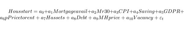
- Mortgageavail is mortgage availability, measured by mortgage loan divided by median home prices in each period,
- Mr30 is conventional 30-year mortgage interest rate,

- CPI is Consumer Price Index,

- Saving is the personal saving rate at the national level,

- GDPR is real GDP in 2005 billion dollars,

- Pricetorent is the ratio of price to rent,
- Hassets is household assets,

- Debt is household debts,

- Mhprice is the median home price,

- Vacancy is the vacancy rate,

Data
This analysis uses quarterly data from the first quarter of 1980 through the fourth quarter of 2010 to estimate the effects of changes in mortgage interest rates on housing starts. The list of variables, their summary statistics, and their sources are presented in Table 1.[29] Data on national and regional vacancy rates, housing starts, property taxes, and ownership rates were obtained from the Census Bureau.[30] The data on down payments and mortgage loans were retrieved from the Federal Housing Finance Agency (FHFA).[31] Data on family income, median home prices, and adjustable mortgage interest rates are from Realtors Research.[32] Data for the rest of the variables are from the Federal Reserve Bank of St. Louis.[33]

Stylized Facts on Housing Starts. The data indicate that housing starts at the national level have been quite volatile since 1960, increasing from 1990 to 2005, before dropping dramatically in the second quarter of 2006 when the housing bubble burst. (See Chart 1.) Housing starts in the fourth quarter of 2010 totaled 539,000 units—its lowest level, with a huge drop from 2,036,000 units in the fourth quarter of 2003. One of the main reasons for this drastic chute is a sharp drop in median home prices.
Regional Housing Starts. The data for housing starts by region, which are available from the first quarter of 1993, indicate that housing starts in the South have exceeded every other region. (See Chart 2.) Mayer and Somerville attribute this to employment and population growth in the South.[34] In decreasing order, housing starts in the Midwest, West, and Northeast closely move together. The lower levels of housing starts in the Northeast and West can be attributed to the tighter land restrictions in these regions.
Mayer and Somerville argue that environmental regulations and development constraints in the Northeast and in California, Oregon, and Washington—a large part of the West—delay home builders’ response to changes in economic conditions and, as a result, to lower levels of housing starts.[35] Land regulations trigger distortions in land and housing prices, which create domino effects on the housing starts.
Randal O’Toole argues:
[A]t a state level the biggest housing bubbles, with prices rising more than 80 percent after 2000 and then dropping by 30 to 60 percent since their peak, were in California, Florida, Maryland, Nevada, and Rhode Island. All these states except Nevada have growth management laws.… New York and District of Columbia had bubbles but did not have growth management. But New York City and Washington, D.C., are both hemmed in by states that used growth management. A few states, such as Minnesota, Montana, and New Mexico, came close to meeting the bubble definition but did not have housing prices rise by the full 50 percent. These states did not have mandatory statewide growth management, but some of their major cities practiced growth management.[36]
O’Toole finds a very close relationship between regions with growth management planning and regions that have observed a bubble burst. He concludes that land-use regulation was the single most important factor in the housing bubble of 2006; therefore, deregulating housing markets could prevent another bubble in the future.[37] Obviously, although land regulations played an important role in creating the bubble in some states, it may not have been the single most important factor, since both demand and supply-side factors were in tandem.
Wendell Cox and Ronald D. Utt argue that advocates of zoning and environmental regulations have been trying to reshape American communities to conform to their smart growth policies. Since the 1970s, fast-growing communities, such as those in California and Oregon imposed more land-use regulations than other states to discourage people from moving to their communities. In the late 1990s, the anti-suburban advocacy and New Urbanism movements began to implement zoning and other forms of land-use regulations to deter growth or limit access to residents and businesses with specific demographic features. To achieve these goals, many communities adopted more restrictive land-use regulations and imposed impact fees on new houses. Minimum lot sizes, growth boundaries, green belts, and other types of regulations added to the cost of a house by creating artificial land shortages, which in turn raised home prices. In fact, land-use regulations decreased housing starts, especially in communities in the West and South with more land-use regulations.[38]
Regional Vacancy Rates. The South has the highest observed vacancy rate among the four census regions. The Midwest, West, and Northeast rank in decreasing order after the South. The vacancy rate in the Northeast exceeded the West and Midwest from 1993 through 2001, but has reversed the trend since 2001. (See Chart 3.) In short, the vacancy rate in the West has moved closely with the vacancy rates in the Midwest and Northeast. The only outlier is the South, which had the highest vacancy rate. One reason besides the land-use restrictions might be the higher population density, as discussed by Haltom and Sarte.[39] Another reason is the higher rent-to-price ratio in the South compared with other regions, as discussed by Sean D. Campbell, Morris A. Davis, Joshua Gallin, and Robert F. Martin.[40] (For more detailed data on the regional disparities in rent-to-price ratios, see Appendix B.)
The South had the highest rent-to-price ratio from 1975 to 2007. This may be attributed to the growth of population and employment in the region, as a result of its growth management plan. The higher employment rate has led to higher demand for real estate, which in turn, has led to the higher rent-to-price ratio in the region.
Regional Sale to Inventory Ratios. The sale-to-inventory ratio at the regional level has been volatile since the early 1990s. (See Chart 4.) However, the sale-to-inventory ratio in the South has exceeded every other region. The Midwest, West, and Northeast rank in decreasing order. The sale-to-inventory ratio has been lower in the Northeast and West compared with the South and Midwest because the housing meltdown hit the Northeast and West more severely than other regions. Furthermore, land use is more heavily regulated in these regions, and many scholars have argued land restrictions have led to higher housing prices among these regions.
A seminal study by Theo S. Eicher uses Census data for 2,730 jurisdictions and 2006 Census public micro sample data. He uses land-use regulations as independent variables, whether imposed by governors and legislators, courts, growth management bodies, or residential buildings. He finds a statistically significant relationship between land restrictions and higher housing prices.[41]
In a similar study, Stephen Malpezzi, Gregory H. Chun, and Richard K. Green analyze the determinants of housing prices with a particular focus on the supply-side determinants such as regulatory and natural constraints. They use a set of regulatory measures including rent controls, land use, zoning regulations, infrastructure policies, and building and subdivision codes. They find that housing prices are related to physical constraint, population, income, and demographic variables and that regulations drive up rents and housing prices. They conclude that moving from less stringent to more stringent regulated areas increases rents from 13 percent to 26 percent and housing prices by 32 percent to 46 percent.[42]
Using 1990 Census population data, Richard K. Green traces the effects of land-use restrictions on housing prices. He uses six land-use restrictions—forbidding mobile homes, minimum lot width requirements, minimum frontage setbacks requirements, minimum street width requirements, sidewalk requirements, and curb and gutter requirements—and a variable indicating whether the community has a written standard for home prices. He finds that an additional 10 feet setback regulation increases housing prices between 6.1 percent and 7.8 percent. Forbidding mobile homes pushes up prices by between 7.1 percent and 8.5 percent, and subdivision requirements for curbs and gutters are associated with higher rents of 10 to 12 percent.[43]
Edward Glaeser argues that restricting housing supply leads to greater volatility in housing prices.[44] He compares the median home prices of Boston with prices in Atlanta. The Atlanta region issues about seven times as many permits as the Boston region. He finds that median housing prices in Boston are higher and more volatile than housing prices in Atlanta, which neither shared the Boston Boom when prices doubled between 1980–1988 nor suffered from Boston’s housing bust when prices lost 50 percent during 1988–1994. He concludes that land-use restrictions lead to higher prices.[45]
In a more recent study, Huang and Tang use data for 300 U.S. cities and examine land-use regulations and land scarcity to see how they are related to housing price cycles between 2000 and 2009. They find that more land-regulated cities experienced greater price booms between January 2000 and June 2006 and greater price declines between June 2006 and July 2009. They argue that the land regulations amplified the boom-bust behavior of the sub-prime mortgage market.[46]
Regardless of the region under investigation and the type of restriction imposed, land-use restrictions can have major impacts on housing prices and price volatility, which in turn can tremendously affect housing starts and sale revenues. As a result, we expect lower sale-to-inventory ratios in more land-restricted areas such as the Northeast and West. (See Chart 4.)
Econometric Results at the National Level. The equation described in the theoretical section was estimated at the national and regional levels to measure the elasticity of housing starts to the conventional mortgage interest rate, controlling for economic fundamentals such as household assets, family income, personal income, real GDP, saving rate, price-to-rent ratio, and the property tax rate. This analysis used four different specifications (Models 1 to 4). The first model relates housing starts to mortgage availability, median home prices, household assets, the S&P index, family income, CPI, savings rate, mortgage interest rate, and business cycle index. The second model uses mortgage availability, price-to-rent ratio, ownership, S&P index, real GDP, CPI, household debt, vacancy rate, mortgage interest rate, and business cycle index. The third model includes mortgage availability, home prices, price-to-rent ratio, real GDP, CPI, vacancy rate, mortgage interest rate, and business cycle. Finally, the fourth model uses all the variables in the third model plus household assets. All variables are in logarithm form. Therefore, the estimated coefficients are elasticities. In addition, all models have been tested for robustness.
The estimated results, presented in Table 2, indicate that the elasticity of housing starts to mortgage interest rate is very small, particularly when compared with economic fundamentals such as real GDP, CPI, and price-to-rent ratio. The results indicate that these independent variables explain more than 88 percent of changes in housing starts.
Because it is important to distinguish between the expected interest rate and nominal interest rate, the CPI level was included in the model. Indeed, because the mortgage interest rate is a nominal interest rate, it is important to modify it for the expected inflation. Therefore, to adjust for the inflation rate, the CPI was included in the model. However, to ensure that independent variables are not correlated, particularly the mortgage interest rate and the CPI, the analysis used the variance inflation factor (VIF) to test for multicolinearity. The VIF test results suggest no colinearity between the mortgage interest rate and the CPI, because VIF > 10. (See table in Appendix B.)
Many economists argue that the presence of Fannie Mae and Freddie Mac in the secondary mortgage market affects the primary mortgage market rate. Lawrence J. White argues the GSEs’ activities cause the interest rates on the confirming mortgages to be about 20–25 basis points lower than the rates on jumbo mortgages.[47] In another paper, W. Scott Frame and Lawrence J. White conjecture that shutting down the GSEs would cause mortgage interest rates to jump 25 basis points.[48] Several econometric studies have found that the interest rates without Fannie and Freddie would be 20–35 basis points higher, but the estimates vary substantially depending on the empirical specification, sample, and time period.[49] Based on these and many other empirical studies we assume that without Fannie and Freddie the housing market for 1980–2010 would have seen mortgage interest rates average 25 basis points higher than what actually prevailed.[50] In fact, this would mean a one-time jump in the mortgage interest rate, which affects the intercept of the regression model, not its slope. Therefore, it is a transitional, short-term effect. The long-run effects on macroeconomic variables are considered in a forthcoming Heritage paper on the economic effects of eliminating the GSEs in a general equilibrium model.[51]
Based on the estimated results of this Heritage study, the average elasticity of housing starts to mortgage interest rate at the national level is 0.20. To illustrate what a 25 basis point increase in the mortgage interest rate can do to the housing starts, we use the elasticity of housing starts to mortgage interest rate, 0.20. Multiplying this elasticity by a 25-basis-point increase in the mortgage interest rate yields a 0.05 percent reduction in the housing starts (0.2 * 0.25 = 0.05). In other words when compared with changes in other fundamentals, such as real GDP, or CPI, a small upward shift in the conventional mortgage interest rate has a minor, negative, one-time effect on housing starts. As a matter of fact any small change in real GDP or consumer price index (CPI) would affect housing starts much more than any change in mortgage interest rates. For instance, a 2 percent increase in CPI reduces the housing starts by 8 to 10 percent, which is substantially larger than the effects of the changes in mortgage interest rates that would result from shutting down Fannie and Freddie.
The results of this study are in accordance with those of Christian Pierdzioch, Jan-Christoph Rulke, and Georg Stadtmann, who found that expected housing starts are mainly affected by macroeconomic fundamentals, such as real GDP, CPI, and expected inflation, not the short-term mortgage interest rate, which plays a very small role in shaping housing starts.[52]
Econometric Results at the Regional Level. It is important to examine regional results in this study because different regions have different land-use regulations, population densities, and growth management plans. Across regions, we may observe that changes in mortgage interest rates have different effects on housing starts.
Furthermore, the sum of regional elasticities does not add up to the national elasticity for many reasons. First, the independent variables in the regression models in the national and regional levels are different, so the elasticities will be different. Second, even if the independent variables were the same, elasticity is not a simple variable like population, in which the total of regional populations equals the national population. The sum of regional elasticities—the percentage change of housing starts to percentage change of mortgage interest rates—does not necessarily add up to the national level. Third, many empirical studies have found differences between regional elasticities and national elasticities.
The Census Bureau divides the U.S. into four main geographic regions: West, Midwest, South, and Northeast. This classification is based purely on geography, not demographics or economics. Because the Census Bureau has historically released regional-level data for empirical studies, they continue to release the data in the same format to avoid disrupting the time series data on housing starts.
This section measures the effects of changes in mortgage interest rates compared with other economic fundamentals on housing starts at the regional level. The estimated results indicate that housing starts in the Northeast are elastic to mortgage loan availability, rent, personal income, real GDP, and property tax rates. (See Table 3.) However, the most important factors shaping housing starts in the Northeast are property tax rate, personal income, and real GDP.
The results also indicate that the most important factors in shaping housing starts in the Midwest are family income, personal income, real GDP, and property tax rate. Interestingly, the elasticity of housing starts to conventional mortgage interest rates in both the Midwest and the Northeast is 0.02.
For the South, the most important factors driving housing starts are family income, personal income, and property tax rate. However, the elasticity of housing starts to mortgage interest rates in the South is larger than in the Northeast and Midwest. In other words, changes in conventional mortgage interest rates affect housing starts in the South more than housing starts in the Northeast and Midwest. As discussed earlier, this might be the result of higher population density and growing employment in the South.
In the West and the South, housing starts are more sensitive to family income and property tax rate. The econometric results of this study indicate that the elasticity of housing starts to conventional mortgage interest rate in the South and West equals 0.04. In other words, a 25-basis-point increase in the conventional mortgage interest rate, as a result of shutting down Fannie Mae and Freddie Mac, reduces housing starts by only 0.01 percent in the South and West, and by 0.005 percent in the Northeast and Midwest.[53] These results closely match those of Gupta, Jurgilas, Kabundi, and Miller who find that the response of housing starts in the West differs from the national response and other regions.
All in all, despite regional disparities in income and land-use regulations, the elasticities of housing starts to mortgage interest rates are very small for all regions, particularly when compared with economic fundamentals such as GDP, family income, and property tax rates. In other words, changes in economic fundamentals will affect housing starts much more than changes in conventional mortgage interest rates.
Conclusion
The results of this empirical study suggest that conventional mortgage interest rates play a minor role in shaping housing starts at both the national and regional levels. The results are in accordance with those of Ewing and Wang, who find that mortgage interest rates play a minor role in housing starts. The regional results closely match those of Gupta, Jurgilas, Kabundi, and Miller who find that housing starts respond differently in the West. The results also indicate that the South and West are more responsive to changes in mortgage interest rates than the Midwest or Northeast because the South and West have more land-use restrictions and environmental regulations, which intensify the responsiveness of house builders to changes in mortgage interest rates. The South also reacts differently than other regions to changes in mortgage interest rates because of its higher population density. Therefore, shutting down Fannie and Freddie will likely affect the South and West more significantly than the Northeast and Midwest.
One of the reasons that some studies have found higher elasticity of housing starts to mortgage interest rate is that they have controlled for only a few—or zero—economic fundamentals in their studies. The results of this paper indicate that the economic fundamentals—such as real GDP, CPI, household assets, household debts, family income, and price-to-rent ratio—primarily shape housing starts at the national level. However, in the South and West, personal income, real GDP, and property tax rates drive housing starts. The higher elasticities of housing starts to property tax rates at the regional level suggest that policymakers should exercise more caution in raising property taxes because they may drastically reduce the number of housing starts and residential investment, particularly in the Northeast.
In sum, the results of this study based on 30 years of data cast doubt on the claim that Fannie Mae and Freddie Mac actually increase homeownership at the national and regional levels. Assuming the housing and finance sectors someday return to normal, and that this evidence from the past sheds light on the future, these results indicate that phasing out the GSEs would minimally affect housing starts and home ownership at the national and regional levels—at most a 0.01 percent drop in the housing starts in the South and West and 0.005 percent drop in the Northeast and Midwest.
Indeed, regardless of the level of aggregation or the region, the results of this study confirm that economic fundamentals, not conventional mortgage interest rates, primarily shape housing starts. The government and GSEs are leveraging the wrong instrument because subsidized mortgage interest rates have minimal impact on housing starts at the national and regional levels. Moreover, as discussed by many scholars, land-use regulations play an important role in home price volatility and housing starts because home builders’ beliefs are shaped by the regulatory environment and their investment returns, rather than by mortgage interest rates. Continuing to subsidize the mortgage interest rates is a waste of taxpayers’ money because mortgage interest rates do not significantly influence home builders’ decisions.
- Nahid Kalbasi Anaraki, Ph.D. is a Visiting Fellow for Special Projects in the Center for Data Analysis at The Heritage Foundation.
Appendix A
Summary of the Literature Review
Appendix B
Data