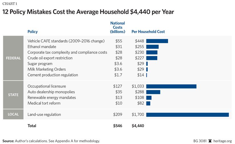
Government policy mistakes raise the prices of the things that Americans buy. An average American household can expect to pay an extra $4,440 each year thanks to just 12 such policy mistakes that have large costs and few benefits.
Local, state, and federal governments are all guilty of enforcing costly laws and regulations. At the federal level, the biggest costs come from vehicle fuel-efficiency standards, which cost consumers $55 billion a year, and the requirement to use corn-based ethanol in gasoline, which costs $31 billion per year. Occupational licensure at the state level costs consumers $127 billion per year. Local land-use restrictions drive up the cost of housing by $209 billion per year.
Altogether, the 12 policy mistakes quantified in this paper cost Americans $546 billion per year or 4.6 percent of total consumption. That is comparable to the Department of Defense budget and 18 times the budget of the National Institutes of Health. It is more than half as much as Americans spend on groceries, and more than the rent paid by every renter in America. It is three times the budget of the State of California. It is more than what 14 million average Americans spend in a year. And we pay it again and again, year after year.
The ban on crude oil exports is a typical policy mistake that costs Americans. While most economists would initially guess that banning exports leads to lower domestic gasoline prices (but also lower income), recent analyses concluded that the opposite is true: American consumers would pay 12 cents less per gallon of gas if the ban were lifted. Section 3 discusses 12 such costly policies, and Appendices A, B, and C give details on the calculations, assumptions, and references behind each estimate.
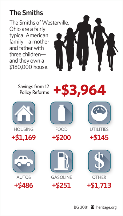
The Smiths of Westerville, Ohio, are a typicalAmerican family, although unlike most Americans they are fictional. They own a $180,000 house and visibly spend $74,000 a year.[1] Due to costly and unnecessary government policies, they spend an extra $200 on food, $145 on utilities, $251 on gasoline, $486 on cars, $1,169 on housing, and $1,713 on consumption in general. That is $3,964 per year that the Smiths cannot spend on college tuition, their leaky garage roof, or the 30th anniversary trip that they keep delaying.
Policymakers at all levels of government can correct policy mistakes by repealing unnecessary regulations, undoing policies that primarily benefit narrow industries, and streamlining bureaucratic processes that impose delays.
Policy Theory
Policy mistakes hurt the U.S. economy in several ways. They lower productivity, increase monopoly power, decrease employment opportunities, shrink incomes, make investment less promising, and raise prices. Although all of these effects are important, this paper focuses on only the impacts on the prices of consumer goods and household budgets, and it considers only 12 policy mistakes. The total cost of failed policymaking is undoubtedly much larger.
Prices and incomes are opposite sides of the same coin. What kind of house can a consumer afford on an income of $60,000 per year? It depends on what prices are. Is a $3 cup of coffee a luxury? It depends, among other things, on how much money coffee-drinkers earn.
Generally, average prices and average incomes rise together (i.e., inflation). As technology increases worker productivity, average incomes rise a little bit faster than average prices (real wage growth).
In many cases, prices are higher than they need to be thanks to poorly designed laws and regulations. With freer markets, prices would fall, and consumers could buy more with every dollar.
How Policy Influences Prices. Policies lead to higher prices when they restrict supply, protect monopolies, add extra requirements to supply, or impose delays on production.
As is taught in Economics 101, lower supply leads to higher prices. Some things are naturally in short supply. Beachfront property in San Diego is limited, so land prices there are high. But restrictions on building make prices even higher. If property owners could legally turn their three-story apartment buildings into 30-story apartment buildings, living at the beach would be cheaper. Incidentally, land values would rise as unit costs fall because each owner would have the option of building up.
In other cases, there is plenty of supply, but government grants monopoly powers to favored corporations, which use their privileged positions to raise prices on consumers and increase their profits. For example, the U.S. sugar program puts strict limits on sugar imports. As a result, American sugar growers can charge higher prices, enriching themselves at the expense of American consumers and killing jobs in the broader food industry.
Some costly laws directly add unnecessary steps to the production process. When corporations pay income taxes, they do not just write a check. They must also gather reams of records. The complexity of the tax code has a lot of drawbacks, and one is that corporations must hire battalions of lawyers and accountants just to file all of the paperwork correctly. Those costs are passed on to customers as higher prices.
Finally, some regulations impose costly delays. Delays often sound harmless to outsiders—what is the problem with waiting a few weeks for the state to process the application for a commercial driver’s license? But for individuals and businesses, delays are very costly, whether they are weeks of lost earnings or months of waiting for a building permit. Delays thus reduce supply by discouraging work, and the added costs are passed on to consumers as higher prices.
Levels of Government. Washington often creates regulations that have large, unforeseen consequences, but policy mistakes at the state and local levels are just as costly. In fact, the federal government, the states, and localities are each responsible for approximately one-third of the cost of poorly designed policies covered in this report.
Each level of government has its own characteristic vice. At the federal level, it is cronyism. Corporate tax complexity is a result of a forest of hometown favors and special exceptions. The sugar program subsidizes one powerful industry; Federal Milk Marketing Orders (FMMOs) another. The costly ethanol mandate probably survives only because of Iowa’s outsized role in picking presidential nominees.
State lawmakers have given in to the temptation to require approval for even the most basic economic activities. For all sorts of economic activities, a person cannot just go about his or her business legally. He or she must first receive permission: permission to drive a commercial vehicle, permission to cut hair, permission to sell cars, or permission to be a school teacher. Each permission slip requirement makes markets more monopolistic and less competitive, thus raising prices, lowering quality, and stunting innovation.
Local governments are suckers for the status quo. They pay lip service to job growth and lower prices, but in practice they block jobs and raise prices when they set strict zoning laws and drag their feet on permitting. In big cities, taxpayer-funded stadiums often seem to be the only major building projects that can be completed quickly.
Who Pays Higher Prices? Everybody who buys goods and services in the U.S. is paying something, but the impact is greater for some.
The most heavily impacted are those who live in cities and suburbs, especially those with strict land-use regulations. Housing is a large share of most budgets, and in high-cost cities housing is often 15 percent more expensive than it would be with more modest land-use regulation. For many families, this means thousands of dollars per year in extra costs due to restrictive local laws and bureaucracy.
High prices strongly impact those who consume a high percentage of their income. The poor, the retired, and young adults tend to consume as much (or more) than they earn, and their consumption is often focused on categories that show up prominently in this report: housing, cars, energy, and food.
Consumer Surplus Versus Higher Prices. Economists might object that measuring only the impact of higher prices misses the additional “deadweight loss” due to regulations. After all, the high price of rent in Seattle affects not only those who pay it, but also those who cannot pay it and must turn down a job offer or spend two hours a day commuting from cheaper suburbs.
Deadweight costs are real and important, but difficult to measure. In the cases of fuel-efficiency standards and cement regulation, published cost estimates directly reported the loss as a decline in consumer surplus, which I used. Elsewhere, the costs are only the visible ones and thus understate the loss to consumers.
This report shows that the costs of policy mistakes are large. If future work takes more policy mistakes into account and can accurately incorporate deadweight loss, the results could be much larger than $546 billion.
Twelve Costly Policies
For each quantifiable policy, this paper reviews some of the recent research on its costs, choses a modest estimate of the size of the cost, and adjusts for inflation to June 2015. Appendix A explains technical details behind the choices and gives full citations for the references.
Costly Federal Policies. Federal policy mistakes are felt by families across the country.
CAFE Standards. Cars and trucks sold in the U.S. are subject to the Corporate Average Fuel Economy (CAFE) standards, a set of Byzantine gas-mileage regulations. The recent round of gas-mileage regulations added about 10 percent to the cost of vehicles, costing the average household $448 per year. Given their high cost, CAFE standards remain one of the least efficient means of controlling pollution.
Thanks to a 2009 regulatory change spearheaded by President Barack Obama, automakers had to increase the fuel efficiency of their fleets by 9 miles per gallon over five years.[2] Not surprisingly, the automakers passed the costs along to car buyers.
Quality-adjusted new vehicle prices declined from 1997 to 2008.[3] After bottoming out in the recession, vehicle prices rose 9.5 percent in six years. If the pre-2008 trend[4] had continued for another seven years, prices would have been 14.8 percent lower in 2014 than they actually were. The average new vehicle costs around $32,500,[5] about $4,500 more than if the price trend had continued.[6]
Researchers anticipated the price increase in papers written before the changes took full effect. This paper uses the median estimate from several models: the loss in consumer surplus is $61 billion per year, which works out to $3,800 per new vehicle. Adding the assumption that businesses pass on only 75 percent of their higher vehicle costs to consumers further attenuates the estimate presented here.
Renewable Fuel Standard. The Renewable Fuel Standard (RFS) mandate to include corn-based ethanol in gasoline hurts U.S. consumers at the gas station and the grocery store to the tune of $255 per year for the average household. By requiring that corn be used inefficiently as fuel, the federal government has raised the prices of fuel and food.[7]
Stephen Holland et al. estimated that the ethanol mandate would raise gas prices 19 cents per gallon by 2022.[8] The Congressional Budget Office (CBO) estimated that the mandate would raise gas prices 13 cents to 26 cents by 2017.
When global food prices spiked in 2008, causing food shortages in very poor countries and hurting consumers worldwide, ethanol mandates drew attention as a potential culprit. Richard Perrin estimated that the ethanol mandate contributed to a rise of 1 percent to 2 percent in food prices, arguing that it was responsible for less than half the spike in global food prices in 2008.
Tax Complexity and Compliance Costs. The federal government levies a wide variety of taxes, some of which are obscenely complicated. The time that individuals and businesses spend saving receipts, filling out forms, and reading 100-page IRS instruction booklets is time not spent on work or leisure.
The complexity of the corporate income tax alone costs $113 billion per year. Suppose that tax reform eliminated deductions, replaced depreciation with expensing, and lowered the marginal tax rate such that compliance costs were cut in half. We do not have estimates of how much of that cost is passed through to consumers as higher prices and how much is absorbed by lower wages or lower profits, but if half of the cost is passed through to consumers, reform would save the average household $230 per year, with the rest of the benefit going to investors and workers.
Corporate tax reform would have economic benefits that far exceed the mere static effect on consumer prices. The distortions introduced by the current system, in which the marginal tax rate is much higher than the average tax rate, misallocate resources and talent and depress investment.[9]
Crude Oil Export Restriction. U.S. oil producers are largely prohibited from exporting crude oil.[10] Many initially assume that the ban lowers U.S. prices of petroleum products. However, the U.S. produces and refines a different mix of oil products than it consumes. As a result, economists at the Brookings Institution and economic consulting firm IHS argue that the crude oil export restriction actually raises consumer prices for gasoline.
Refineries in the Gulf Coast were built to handle heavier crude oil, which is largely imported. The U.S. is now producing higher-quality crude oil, but the old refineries cannot handle all of the new U.S. oil in a cost-effective way. If the export ban were lifted, U.S. producers could sell their high-quality crude for a better price on world markets, U.S. crude oil would be refined more efficiently, and gasoline prices would fall globally—including in the United States.
Removing the export ban would expand production and save American consumers 12 cents per gallon of gas—which adds up to $227 per year for the average household, including savings passed on by businesses.
Sugar Program. The U.S. sugar program sets minimum prices and production controls for U.S. sugar producers and imposes quotas on sugar imported from abroad. American agribusiness benefits at the expense of consumers, sugar growers in poor countries, and American businesses that use sugar.[11]
The sugar program costs consumers $3.6 billion per year. For the average household, that comes to $29 a year.
Milk Marketing Orders. FMMOs are part of a broader U.S. dairy policy intended to maintain the status quo in dairy markets at the expense of consumers. The marketing orders divide the country into regions, setting different prices for wholesale milk in each region.[12] Some dairy farmers benefit, others lose.
Like the Sugar Program, FMMOs cost $29 per year for the average household. The impact is largest on families with small children.
Cement Production Regulation. In theory, environmental regulation should balance costs and benefits. In practice, cost-benefit analysis is only as good as its assumptions, which are often tilted to produce a preferred result.[13]
The Environmental Protection Agency’s systematic imposition of regulation on coal power is well known and could significantly affect the price of fuels, but even minor-sounding regulations on smaller industries can raise prices. For example, Stephen Ryan estimated that the 1990 amendments to the Clean Air Act docked consumers $1.7 billion by raising costs and encouraging monopoly power in the cement industry. The average household may not buy cement directly, but the increased costs of buildings and infrastructure are passed through to them, totaling $14 per year for an average household.
This report does not attempt to incorporate the full cost of environmental regulation. Cement was included as an example because Ryan subjected it to rigorous scholarly review, a rare practice.
Costly State Policies. Bad state policies can cause as much economic damage as bad federal policies.
Occupational Licensure. Thirty percent of Americans now need a license to work legally in their professions.[14] In a few cases—mostly in medical professions—there is clear argument for preventing newcomers from practicing without going through a rigorous pre-examination.[15] However, for most other professions—from barbers to sign language interpreters to schoolteachers—that argument does not apply.
Occupational licensure costs the average American household $1,033 per year, making it one of the most promising areas for reducing prices.
The high cost of licensure is borne out by detailed studies. In a rigorous study, Morris Kleiner et al. estimated that prices of well-child exams are 3 percent to 16 percent lower in states that allow nurse practitioners to prescribe medication than in states that allow only a doctor to prescribe medicine. Since most well-child exams do not involve any prescription at all, even a 3 percent additional cost is quite high. Their research found no difference in health outcomes between states with more rigid regulation and states with more flexible regulation.[16] Licensure is not exclusively a mistake practiced at the state level. Both localities and the federal government license some professions and contribute to higher prices.
Auto Dealership Monopolies. To sell bicycles, a person can order merchandise from bike manufacturers and open a shop. To sell new cars, being born into a family that owns dealerships is helpful. Every state has a phalanx of rules and regulations designed to protect the existing auto dealerships from additional competition. Nor may the car manufacturers sell directly to consumers. They must give the local dealerships a big cut.
As a result of the lack of competition, middlemen jack up the prices of cars by 6 percent or more. For the average new car,[17] this policy adds $1,950 to the price. Most Americans do not buy a new car every year, but over a decade these monopolies will cost the average household an extra $2,880.
Renewable Energy Mandates. Many states mandate that some percent of the state’s electricity be generated from renewable sources. Since most renewable energy sources are not cost-effective, the result is higher prices for consumers. These Renewable Portfolio Standards (RPS) mandates will soon cost the average household $108 per year.
The price effect varies by state, depending on the stringency of the RPS and the local availability of water power, wind, and sunlight. Several states allow renewables to compete on their merits instead of introducing a mandate, incurring no cost at all. Even according to President Obama’s advisers, a typical 2010 government-subsidized wind power project was “more than six times” too expensive to justify on climate-change grounds.[18]
Medical Tort Reform. Health care is riddled with inefficiencies and redundancies. One example is medical malpractice liability, through which potentially devastating awards increase the use of unnecessary procedures. The CBO estimated that tort reform would save 0.5 percent of all medical spending—$82 a year for the average household. Since medical costs are often paid indirectly through insurance premiums and taxes, the savings would work through the system in different ways.
Costly Local Policies. Local land-use regulations can cost families even more than bad federal or state policies.
The city council has as much influence on a person’s cost of living as the federal government. Local governments regulate housing, which is the largest expense for most families. In total, Americans pay about $209 billion a year extra for housing due to overregulation of land use. For the average household, the cost is $1,700 a year, but the cost is distributed very unequally. Rural families and those living in less-regulated cities are unharmed. Those in expensive metro areas are taken to the cleaners, frequently for over $5,000 per year.
Land-Use Regulation. Land-use regulation is not the only mistake that local governments make, but it is certainly the most costly. In the past half-century, local governments have internalized the harmful ideas that cities and suburbs ought to be “planned” by experts and that new construction generally imposes a net cost on other residents.
As a result, zoning boards, planning boards, town councils, environmental review boards, neighborhood commissions, historic preservation societies, and even concerned neighbors routinely delay or block much potential construction in high-cost cities and suburbs.
Land-use regulation takes several forms:
- Zoning laws. Zoning laws regulate how land can be used (commercial, residential, or industrial) and how dense it can be (e.g., height and lot size). Zoning laws are usually designed to preserve the past and block the natural transitions among different uses of land. Some types of use impose major burdens on neighbors (e.g., chemical factories), but all sorts of development have generally positive effects on the surrounding area by lowering prices and creating job and commerce opportunities. Zoning should only restrict uses that clearly fail a cost-benefit test. For most other uses—such as apartment buildings, warehouses, and offices—government restrictions are inappropriate.
-
NIMBYism. Local governments often face pressure from citizens who do not mind construction in theory, but want it “not in my back yard.” Neighborhood review is appropriate for government projects that propose to alter public spaces such as roadways, but neighbors should not be allowed to veto private building projects simply because they dislike them.
Bureaucrats empower NIMBYists by enacting complex approval processes for projects and setting zoning requirements so that any economically feasible project needs to receive a variance from the written requirements. Each additional permit and paperwork barrier allows opponents of affordability to keep rent high. Private arrangements, such as homeowners’ associations, often have the same effect, giving homebuyers the choice of agreeing to burdensome rules or writing off a desirable neighborhood.
-
Environmental review delays. A primary cost of environmental review, which often involves state and federal agencies, is the delay it imposes on construction projects. While a delay may appear trivial to outsiders, it represents time that funds must sit, earning nothing, waiting for the right signatures. The delays add costs to some projects and forestall others altogether, decreasing the supply of structures and raising rents.
Environmentally motivated restrictions on construction often have consequences that are the opposite of their intent. When cities are artificially expensive, more farmland is turned into residential developments than would be the case in a free market.[19] Where building is difficult, prices rise sharply when demand rises. Those prices make life more expensive for homebuyers, renters, and businesses. Businesses pass the costs on to customers as higher prices.
Ed Glaeser and Joseph Gyourko noted that “there is as much land per household in San Diego as there is in Cleveland,” but prices are much higher in San Diego thanks to zoning and “other land use restrictions.”[20] In another paper, with Raven Saks, they showed that housing prices in New York City far outpaced construction costs only after 1980. Until then, housing prices were kept in check by a much higher rate of permitting.[21]
Keith Ihlanfeldt found that the addition of each new form of regulation added 7.7 percent to the price of houses in Florida.[22] Haifang Huang and Yao Tang found that higher regulation led to stronger boom-and-bust housing cycles, which is to be expected when supply cannot respond to demand.[23]
In an eye-popping study, Chang-Tai Hsieh and Enrico Moretti estimated that if just three cities—New York, San Francisco, and San Jose—adopted more modest but typical U.S. land-use regulations, national income would rise 10 percent (about $1.7 trillion) as people moved from low-productivity to high-productivity cities.
Calculations presented in Appendix B show that residents of a typical city in the high-cost coastal areas of the U.S. would pay 9 percent less in rent and 20 percent less for the costs of homeownership if the city adopted regulatory policies that are typical of the rest of the country. On the flip side, if cities with modest regulation add more, they can anticipate rising prices.
This paper does not consider how higher commercial real estate costs are passed on to customers as higher prices, but anyone who has gotten a sandwich in New York knows that those costs are real. If they could be accurately estimated, the total estimated damage done by overregulation of land would be substantially higher.
Results
The costs add up. Taken together, these 12 policy mistakes cost the average American household $4,440 per year. The costs are split roughly equally between localities (38 percent), states (34 percent), and the federal government (28 percent).
The most costly policy mistakes are, not surprisingly, those that affect the largest markets. Housing is the largest item in most family budgets, so restrictions on housing supply are unsurprisingly the most costly policy mistakes. Land-use restrictions seriously increase housing costs in most American metropolises as well as costs for commercial space, although this report does not estimate the latter. Occupational licensure covers about 30 percent of workers, raising wages for insiders and lowering wages for those excluded from the market. Services in education, health, personal care, and many other areas are more expensive due to the costs of licensure. CAFE standards and auto dealership monopolies have large impacts on a large market because transportation is second to housing in most family budgets.
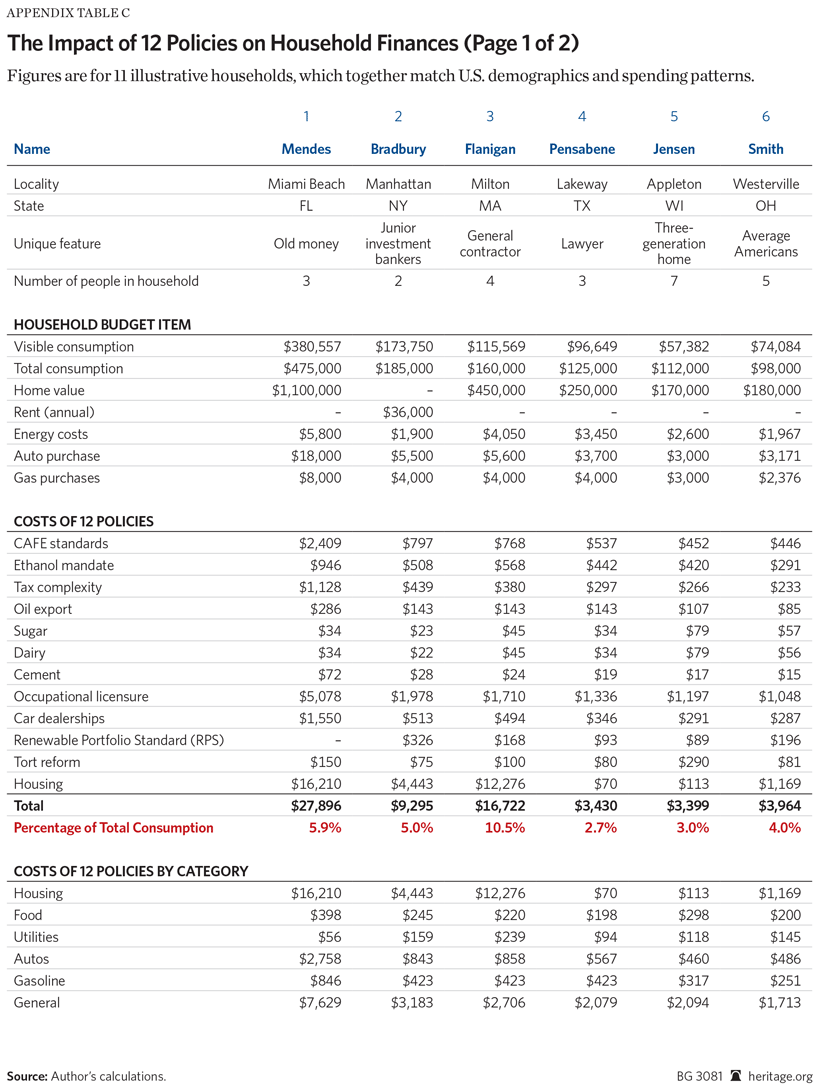
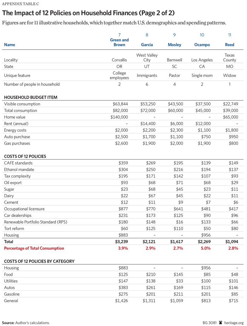
To make the results accessible and to examine distributional effects, Appendix Table C presents the effects of the 12 policy mistakes on 11 American households. The households are fictional, but accurately represent American demographics, geography, and spending.
The Smiths, from Westerville, Ohio, were introduced earlier in the paper. They spend 4 percent of their total consumption on higher prices due to the 12 policy mistakes—slightly below average. Their total consumption equals the national average for households. They own an average-priced home and live in a metropolitan area (Columbus) with land-use regulations near the median.
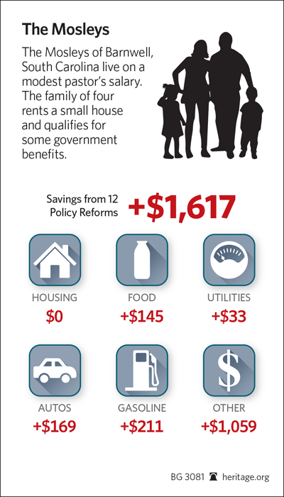
The family that paid the least due to bad policies is the Mosley family of Barnwell, South Carolina. Living on a pastor’s salary makes them working class. The family has a visible consumption of $43,500 per year and qualifies for some government benefits. They are only the third-poorest family in my sample, but with four mouths to feed they live simply. Since small-town Barnwell has plenty of land and few restrictions, land-use regulation does not cost them anything. South Carolina also has a very mild RPS, which adds just $12 to their annual electric bill. Even so, the costs of occupational licensure, corporate tax complexity, the ethanol mandate, and other broad policies are passed on to them as higher prices. They pay an extra $1,600 a year due to the bad policies, 2.7 percent of their total consumption.
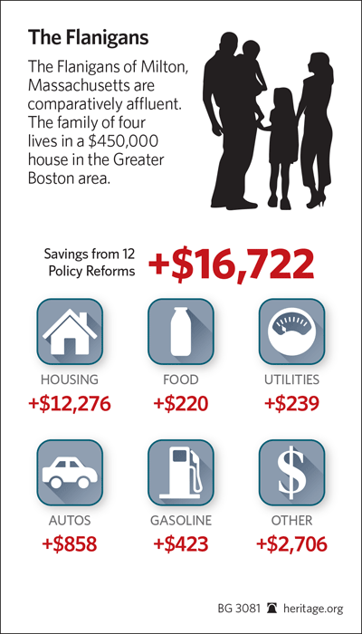
At the other end of the scale are the affluent Flanigans of Milton, Massachusetts. Higher prices due to bad policies eat up 10.5 percent ($17,000) of their total consumption. The Flanigans spend a lot on housing by national standards, but not by Greater Boston standards. Their $450,000 house was not built to be expensive. It just became that way over the past 50 years as demand grew and supply stagnated. Greater Boston’s highly restrictive land-use laws add $12,000 to the Flanigans’ annual housing costs. They face higher electricity prices than the Mosleys due to Massachusetts’ 15 percent renewable energy target.
The Smiths, Mosleys, Flanigans, and the rest of the fictional households are presented in Appendix Table C.
Policy Conclusions
Policymakers at all levels of government can improve policies to lower prices for consumers. Even if Washington will not act, state and local leaders can ease the cost of restrictive laws and regulations.
In several cases, policymakers should simply repeal the misguided or cronyist policies. The sugar program, FMMOs, and licensing for most nonmedical professions exist to benefit the few at the cost of the many and should be removed.
Other policies, such as licensure for medical occupations, can be reformed to fulfil their purposes while imposing less of a cost. Licenses should be cheap, easy to apply for, and have minimal bureaucratic turnaround time. Continuing education requirements can be eased or removed, lowering the cost of working for those who are in active practice. Scope of practice can be expanded, such as allowing nurse practitioners to prescribe medication.
The environmental policy mistakes in this report, such as CAFE standards, are vastly less efficient than market-based policies. These areas should be reevaluated, taking into account a broader range of costs and benefits than were originally considered.
Reforms of local land-use laws are close to home and can even become personal. Local officials often have a great deal of discretion in granting variances from zoning laws, and they must live with angry voters. Local leaders can make life less expensive for their residents by adopting less stringent rules, reducing paperwork, and giving projects the benefit of the doubt.
This report has covered merely 12 policy mistakes. Other, similar mistakes have costs as well, but those costs have not been quantified as fully. For example, the maritime Jones Act makes almost everything more expensive for residents of Alaska, Hawaii, and Puerto Rico, but few attempts have been made to measure the full cost. Small business licensing regimes probably have similar effects on prices as occupational licensure. Policymakers can benefit consumers whenever they remove barriers to competition and simplify regulation.
—Salim Furth, PhD, is Research Fellow in Macroeconomics in the Center for Data Analysis, of the Institute for Economic Freedom and Opportunity, at The Heritage Foundation. The author thanks Robert Arons, Michael Hendrix, Mark Jacobsen, Morris Kleiner, Daniel Sumner, and Weifeng Zhong for valuable comments. Christa Deneault, Kirby Lawrence, and Max Lies provided research assistance.
Appendix A: Cost Estimate Details for Federal and State Policy Mistakes
CAFE Standards
The market for vehicles is extremely complex, and good models are necessarily complicated as well. To make estimates comparable, I isolated the effect on consumer surplus or welfare estimated in each paper, adjusted it to conform to a 1.1 gallons per 100-mile increase in the CAFE fuel-efficiency standard,[24] and adjusted for inflation.[25] Appendix Table 1 shows the astounding range of estimates.
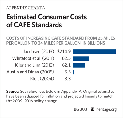
The methodologies gave few clues as to the reason for the wide variance in estimates. Even the authors did not seem to have a sense of whether their estimates were large or small. For example, Andrew Kleit clearly disliked the CAFE regime and seemed to think his estimate was large. Kate Whitefoot et al. present their paper as evidence that costs are not very high, yielding “estimates for [corporate] compliance costs that are nine times lower” than another approach. (Their corporate compliance costs were low because the corporations can pass the costs almost fully to consumers.) It is clear that the cost estimates are much larger after 2009, when the Obama Administration’s tightening of CAFE standards was under way and the marginal gallon-per-mile was falling.
In calculating the applied estimates in Appendix Table 1, I made two choices that biased the findings toward zero. I did not adjust the estimates for population growth or economic growth, only for inflation. I also assumed that each gallon-per-mile increment in fuel economy is equally costly, although increasing marginal cost is a more reasonable assumption. For the point estimate, I used Thomas Klier and Joshua Linn’s estimate, not because I endorsed their methodology above others, but because it was the most modest of the Obama-era estimates.
Klier and Linn’s estimate implies a new-vehicle price impact of $3,800—five times larger than the impact expected by the Obama Administration.[26] The nominal price index trend reviewed in the main text suggests that it is quite reasonable to believe that new regulations have added $3,800 to the cost of a new vehicle. The price trend relative to overall consumer inflation is even more striking in that it implies that quality-adjusted vehicle prices are 21.3 percent above trend.
Mark Jacobsen, whose paper was the clearest and most richly modeled, found that the CAFE standard costs “fall disproportionately on low-income households” as the costs are passed through to the used-car market.
References
Andrew Kleit, “Impacts of Long-Run Increases in the Fuel Economy (CAFE) Standard,” Economic Inquiry, Vol. 42, No. 2 (April 2004), pp. 279–294.
David Austin and Terry Dinan, “Clearing the Air: The Costs and Consequences of Higher CAFE Standards and Increased Gasoline Taxes,” Journal of Environmental Economics and Management, Vol. 50, No. 3 (November 2005), pp. 562–582, http://www.colby.edu/economics/faculty/thtieten/ec476/Austin.pdf (accessed September 17, 2015).
Kate Whitefoot, Meredith Fowlie, and Steven Skerlos, “Product Design Responses to Industrial Policy: Evaluating Fuel Economy Standards Using an Engineering Model of Endogenous Product Design,” University of California Berkeley, Energy Institute at Haas Working Paper No. 214, February 2011, https://ei.haas.berkeley.edu/research/papers/WP214.pdf (accessed September 17, 2015).
Thomas Klier and Joshua Linn, “New-Vehicle Characteristics and the Cost of the Corporate Average Fuel Economy Standard,” The RAND Journal of Economics, Vol. 43, No. 1 (Spring 2012), pp. 186–213, http://www.jstor.org/stable/23209303 (accessed September 17, 2015).
Mark R. Jacobsen, “Evaluating US Fuel Economy Standards in a Model with Producer and Household Heterogeneity,” American Economic Journal: Economic Policy, Vol. 5, No. 2 (May 2013), pp. 148–187.
Renewable Fuel Standard
I used Stephen Holland et al.’s estimate of the impact of the RFS ethanol mandate on gas prices (19 cents per gallon or 7 percent of fuel costs). It coincided with the midpoint of the CBO’s range of impacts.
To allocate the gasoline cost, I used 7 percent of expenditure on “gasoline and motor oil” in the national income and product accounts (NIPA) consumption data. This is likely a low estimate because it misses the indirect cost to consumers of higher fuel prices paid by businesses and passed on in higher prices.
For the food price impact, I had considerably less guidance. The lowest estimates, such as the CBO’s estimate, absolve ethanol of complicity in the large increase in global food prices. The highest attribute the entire rise to ethanol. Richard Perrin’s estimate (1 percent to 2 percent of food costs) was moderate, and he wrote with the tone of a skeptic of a large ethanol impact. I used the low end of his range.
I allocated the percent increase in food prices directly to households as a percent of food-at-home consumption plus 24 percent of food-away-from-home spending. Using only a quarter of expenditures on food away from home reflects the relative share of farm and agribusiness earnings associated with the food-away-from-home “food dollar.”[27]
References
Stephen P. Holland et al., “Some Inconvenient Truths About Climate Change Policy: The Distributional Impacts of Transportation Policies,” Massachusetts Institute of Technology, Center for Energy and Environmental Policy Research, August 2011, http://web.mit.edu/ceepr/www/publications/workingpapers/2011-016.pdf (accessed September 17, 2015).
Richard K. Perrin, “Ethanol and Food Prices—Preliminary Assessment,” University of Nebraska–Lincoln, Faculty Publications: Agricultural Economics, Paper 49, April 2008, http://digitalcommons.unl.edu/cgi/viewcontent.cgi?article=1049&context=ageconfacpub (accessed September 17, 2015).
Jayson L. Lusk, “Distributional Effects of Selected Farm and Food Policies: The Effects of Crop Insurance, SNAP, and Ethanol Promotion,” George Mason University, Mercatus Center Working Paper, April 2015, http://mercatus.org/publication/farm-food-policies-crop-insurance-snap-ethanol-promotion (accessed September 17, 2015).
Thomas E. Elam, “Food Costs Are Eating American Family Budgets,” FarmEcon, January 7, 2013, http://www.farmecon.com/Documents/Food%20Spending%20Eating%20American%20Budgets%20ELAM%201-8-13.pdf (accessed September 17, 2015).
Federal Corporate Income Tax Complexity and Compliance
I limited consideration to the corporate income tax. Other taxes, including state and local taxes, impose substantial burdens as well, and including their effects and interactions would amplify this estimate. I assumed that a simplified tax would occupy half as much time and money as the current code.
I found little empirical guidance on the pass-through of tax compliance costs to prices. There is a large literature on the incidence of corporate income taxation, which finds that the costs are mostly borne by capital and labor. However, that literature assumes that corporate tax rates are equal across firms and industries. That is a simplification and clearly untrue with compliance costs, which are highly idiosyncratic. Furthermore, unlike the literature on universal corporate taxes, the literature on firm-specific and industry-specific costs suggests that pass-through to prices is substantial.[28] For an industry-specific cost, the logic is clear: The industry is large in its own product market, but small in capital and labor markets. Thus, it cannot stiff labor or capital in the long run and must raise prices to pay its factors of production. In the case of firm-specific costs, a firm with above-average costs could not survive in a purely competitive market, so such costs are indicative of some measure of market power. Market power enables such firms to pass costs through to consumers at a higher rate than in competitive markets.[29] Since industry-specific and firm-specific costs can both be passed through to consumers at substantial rates, I used 50 percent as the pass-through rate.
George Contos et al. estimated the cost of corporate income tax compliance at around $100 billion in 2009. The IRS Taxpayer Advocate estimated that completing corporate and individual income taxes required a total of 6.1 billion hours annually. Laffer et al. estimated that the hours were split almost evenly between the corporate and individual income taxes, and they estimated the cost of the corporate income tax at $168 billion in 2008.
I directly used Contos et al.’s preferred specification.[30] The estimate comes from the Business Taxpayer Burden Model and monetizes time spent on tax preparation at different rates for different corporations (larger companies pay higher salaries and are more likely to have dedicated tax accountants), aggregating the results for a national total.
References
George Contos et al., “Taxpayer Compliance Costs for Corporations and Partnerships: A New Look,” Internal Revenue Service, 2012, http://www.irs.gov/pub/irs-soi/12rescontaxpaycompliance.pdf (accessed September 17, 2015).
Taxpayer Advocate Service, “The Complexity of the Tax Code,” 2012 Annual Report to Congress, Vol. 1, http://www.taxpayeradvocate.irs.gov/2012-Annual-Report/downloads/Most-Serious-Problems-Tax-Code-Complexity.pdf (accessed September 17, 2015).
Arthur B. Laffer, Wayne H. Winegarden, and John Childs, “The Economic Burden Caused by Tax Code Complexity,” Laffer Center, April 2012, http://www.laffercenter.com/wp-content/uploads/2011/06/2011-Laffer-TaxCodeComplexity.pdf (accessed September 17, 2015).
Crude Oil Export Restriction
IHS and NERA, two major economic consulting firms, analyzed the effects of lifting the crude oil export ban and found very similar results. IHS (on contract with parties with a direct interest in oil exports) estimated that lifting the ban would lower gasoline prices by 12 cents per gallon when production feedback effects were included. NERA (on contract from the Brookings Institution’s Energy Security Initiative) likewise estimated 12 cents in its “high oil” scenario. The consultancies estimated price declines of 8 cents and 9 cents in less ambitious scenarios, respectively.
IHS estimated $418 billion in consumer savings over 15 years. For aggregate figures, I simply divided 418 by 15. For household-level figures, I computed the percent increase in fuel prices represented by 12 cents per gallon at 2014 prices (3.6 percent) and applied it to household expenditures on “gasoline and motor oil.”
Reporting on NERA’s findings, Charles Ebinger and Heather Greenley noted that the price benefit is not expected to be permanent unless oil reserves are larger than those currently contained in their model. All studies of the issue noted that the consumer price benefit is a small part of the overall economic benefit.
A 2015 study by the U.S. Energy Information Administration (EIA) used the National Energy Modeling System to estimate the impact of lifting the ban on crude oil exports. It surprisingly found that exports do not increase—and even decrease very slightly in 2025—if the export ban is lifted.[31] There are also no effects on domestic prices. In the high-resource cases, the study did find that exports increase and are accompanied by a drop of 3 cents or 4 cents per gallon in gasoline prices. However, even in the high-resource cases, the study predicted that U.S. production will barely be affected by the availability of export markets. An Institute for Energy Research blog post explains that the discrepancy is due to unnecessarily high transportation costs in the EIA study.[32]
References
IHS, “US Crude Oil Export Decision,” IHS Energy/IHS Economics Report, 2014, https://www.ihs.com/info/0514/crude-oil.html (accessed September 17, 2015).
Charles K. Ebinger and Heather L. Greenley, “Changing Markets: Economic Opportunities from Lifting the U.S. Ban on Crude Oil Exports,” Brookings Institution, September 9, 2014, http://www.brookings.edu/blogs/planetpolicy/posts/2014/09/09-us-crude-oil-exports-ebinger-greenley (accessed September 17, 2015).
U.S. Energy Information Administration, “Effects of Removing Restrictions on U.S. Crude Oil Exports,” September 2015, http://www.eia.gov/analysis/requests/crude-exports/pdf/fullreport.pdf (accessed October 26, 2015).
Sugar Program
Four estimates of the impact of the sugar program put the cost between $2.6 billion and $4.2 billion in 2015 dollars. I used $3.6 billion, the midpoint of the range estimated in a rigorous study by John Beghin and Amina Elobeid. Because sugar costs disproportionately hit poorer families, I allocated the cost to households by headcount instead of food-at-home consumption.
In a dissenting estimate, the U.S. International Trade Commission (USITC) estimated that the program costs consumers only $0.28 billion per year. The gap apparently arises because the USITC predicts that liberalization would lead to a 19 percent drop in the price of imported sugar and a 6 percent drop in the price of retail sugar.[33] By contrast, Beghin and Elobeid predicted a 33 percent drop in both the commodity-market price and retail price,[34] as well as smaller price declines in various grocery items that contain sugar. It is not clear why the USITC did not think that free trade would equalize U.S. and world prices, which were less than half of the U.S. price in July 2015.[35]
References
John C. Beghin and Amani Elobeid, “Impact of the U.S. Sugar Program Redux,” Iowa State University, Department of Economics Working Paper No. 13010, May 2013, https://www.econ.iastate.edu/research/working-papers/p16172 (accessed September 17, 2015). This paper has since been published in Applied Economic Perspectives and Policy, Vol. 37, No. 1 (March 2015), pp. 1–33.
U.S. International Trade Commission, “The Economic Effects of Significant U.S. Import Restraints: Eighth Update,” U.S. International Trade Commission, Investigation No. 332–325, December 2013, http://www.usitc.gov/publications/332/pub4440.pdf (accessed September 17, 2015).
Michael K. Wohlgenant, “Sweets for the Sweet: The Costly Benefits of the US Sugar Program,” American Enterprise Institute, 2011, http://www.aei.org/wp-content/uploads/2011/11/-sweets-for-the-sweet-the-costly-benefits-of-the-us-sugar-program_153001980761.pdf (accessed September 17, 2015).
Promar International, “US Sugar Policy Is Costing Consumers an Extra $4 Billion Annually,” October 19, 2011, http://sugarreform.org/wp-content/uploads/2011/07/U-S-Sugar-Policy-and-Consumer-Costs-October-2011.pdf (accessed September 17, 2015).
U.S. General Accounting Office, Sugar Program: Supporting Sugar Prices Has Increased Users’ Costs While Benefiting Producers, June 2000, http://www.gao.gov/archive/2000/rc00126.pdf (accessed September 17, 2015).
Milk Marketing Orders
Hayley Chouinard et al. summarized four previous papers on the consumer price impact of Federal Milk Marketing Orders. Averaging across the papers, they found that fluid milk is 15.5 percent more expensive with FMMOs. Among processed dairy products, the price impacts varied between 1.5 percent cheaper and 3 percent more expensive.
Prices of dairy products fluctuate for various reasons, so the price impact may be lower or higher at any given time. Xiaowei Cai and Kyle Stiegert show that milk margins have fluctuated within the same range from the late 1990s to 2012 for the three states they studied.
Chouinard et al. estimated the total consumer burden of FMMOs using scanner data. However, their estimates included implausibly high milk consumption: about 4 gallons per week for the average household. Instead of relying on their very high estimate of the consumer impact, I directly applied the 15.5 percent price effect on fluid milk to the “fresh milk” category in the NIPA underlying detail consumption tables. Since cheese represents the largest nonfluid dairy expenditure category, I applied the 0.5 percent decrease in the price of cheese to the NIPA concept of “processed dairy products.”
References
Hayley H. Chouinard et al., “Milk Marketing Order Winners and Losers,” Applied Economic Perspectives and Policy, Vol. 32, No. 1 (Spring 2010), pp. 59–76.
Xiaowei Cai and Kyle Stiegert, “Economic Analysis of the US Fluid Milk Industry,” Applied Economics Letters, Vol. 20, No. 10 (2013), pp. 971–977.
Portland Cement Regulation
I incorporated Stephen Ryan’s estimate of cement regulation consumer surplus, which is $63 million per market in his lower-bound scenario.[36] Multiplied by 27 regional markets that is about $1.7 billion. I assumed Ryan was using 2011 dollars, and I allocated the cost proportionately according to total consumption. A recent working paper by Nathan H. Miller, Matthew Osborne, and Gloria Sheu confirmed that the costs of Portland cement regulation are largely passed on to consumers due to the industry’s concentration.
References
Stephen P. Ryan, “The Costs of Environmental Regulation in a Concentrated Industry,” Econometrica, Vol. 80, No. 3 (May 2012), http://people.hss.caltech.edu/~mshum/gradio/papers/ryan.pdf (accessed September 17, 2015).
Nathan H. Miller, Matthew Osborne, and Gloria Sheu, “Pass-Through in a Concentrated Industry: Empirical Evidence and Regulatory Implications,” February 10, 2015, http://www.nathanhmiller.org/cement-ptr-15.02.04.pdf (accessed September 23, 2015).
Occupational Licensure
Morris Kleiner estimated that the cost of licensure could be as high as $217 billion, given a 15 percent wage premium associated with licensure.[37] In three recent papers, Kleiner and his co-authors have used superior data sources to refine their estimates of the wage premium. Kleiner and Alan Krueger estimated the wage premium at 11 percent to 19 percent based on a telephone survey that they designed specifically for the purpose. Maury Gittleman and Kleiner estimated the wage premium at zero to 12 percent using the National Longitudinal Survey of Youth, depending on the specification. Gittleman, Mark Klee, and Kleiner further improved on that result by using the Survey of Income and Program Participation, which had a specific module on licenses and certification. They found that licensure is associated with a 5 percent to 12 percent wage premium.
I used 8.8 percent, equal to the premium that Gittleman, Klee, and Kleiner estimated in an appendix specification that distinguished required licenses and certifications from nonrequired ones at the two-digit industry level. Plugging the 8.8 percent premium into the formula from Kleiner yields a national cost estimate of $127 billion.
The components of this calculation are not quite internally consistent. The premium estimate is from 2008 and covers a smaller share of workers than the rest of the calculation. The calculation is approximate, but falls in the middle of the range suggested by the ongoing research program.
An extensive literature on occupational licensure exists, but I refrain from reviewing it here.
References
Morris M. Kleiner, “Reforming Occupational Licensing Policies,” Brooking Institution Discussion Paper No. 2015-01, March 2015, http://www.brookings.edu/research/papers/2015/01/28-reforming-occupational-licensing-policies-kleiner (accessed September 17, 2015).
Morris M. Kleiner and Alan B. Krueger, “Analyzing the Extent and Influence of Occupational Licensing on the Labor Market,” Journal of Labor Economics, Vol. 31, No. 2, The Princeton Data Improvement Initiative Part 2 (April 2013), pp. S173–S202, http://www-test.hhh.umn.edu/people/mkleiner/pdf/Final.occ.licensing.JOLE.pdf (accessed September 17, 2015).
Maury Gittleman, Mark A. Klee, and Morris M. Kleiner, “Analyzing the Labor Market Outcomes of Occupational Licensing,” Federal Reserve Bank of Minneapolis Research Department Staff Report No. 504, October 2014, https://www.minneapolisfed.org/research/sr/sr504.pdf (accessed September 17, 2015).
Maury Gittleman and Morris M. Kleiner, “Wage Effects of Unionization and Occupational Licensing Coverage in the United States,” National Bureau of Economic Research Working Paper No. 19061, May 2013, http://www.nber.org/papers/w19061 (accessed September 17, 2015).
Morris M. Kleiner et al., “Relaxing Occupational Licensing Requirements: Analyzing Wages and Prices for a Medical Service,” National Bureau of Economic Research Working Paper No. 19906, February 2014, http://www.nber.org/papers/w19906 (accessed September 17, 2015).
Auto Dealership Monopolies
Gary Lapidus estimated that information technology, if freed from legal constraints, would generate 14 percent cost reductions in supply chain improvements, online sales, and make-to-order retailing. Consumers would pay about 8 percent less, with the other savings taking place internally. It is possible that some of these savings, especially the internal supply-chain improvements, have taken place despite the monopolies, but custom-ordering from manufacturers is still impossible.
A generation ago, Robert Rogers estimated that “relevant market area” entry restrictions raised prices of Chevrolets by 6 percent, although the estimate was imprecise. Frank Mathewson and Ralph Winter found that prices were zero to 10 percent higher in more regulated markets during the era when market area exclusivity regulations were spreading.
Laura Nurski and Frank Verboven estimated that banning exclusive dealing in Belgian auto dealerships would benefit consumers 867 euros per household. Extrapolated to the U.S., that would be about $150 billion or 23 percent of all U.S. spending on vehicles. Gerald Bodisch reported that Brazilian customers pay 6 percent less for custom-ordered General Motors Celtas than for Celtas distributed traditionally.
I use 6 percent as an estimate of the impact of restrictions on auto sales, a figure broadly in accordance with research from different times and places. The estimate is applied directly to new and used vehicle purchases by households, since used car prices closely track changes in new car prices. I assume that businesses can pass on 75 percent of the cost of new vehicles at the margin, and I assume away any effect on used vehicle purchases by businesses. I allocate passed-through business costs to households in proportion to total consumption.
References
Gary Lapidus, “Gentlemen, Start Your Search Engines,” Goldman Sachs Investment Research, January 2000.
Robert P. Rogers, “The Effect of State Entry Regulation on Retail Automobile Markets,” Federal Trade Commission, Bureau of Economics Staff, January 1986, https://www.ftc.gov/sites/default/files/documents/reports/effect-state-entry-regulation-retail-automobile-markets/231955.pdf (accessed September 17, 2015).
Frank Mathewson and Ralph Winter, “The Economic Effects of Automobile Dealer Regulation,” Annales d’Économie et de Statistique, No. 15/16 (July–December 1989), http://www.jstor.org/stable/20075766 (accessed September 17, 2015).
Laura Nurski and Frank Verboven, “Exclusive Dealing as a Barrier to Entry? Evidence from Automobiles,” Center for Economic Studies Discussion Paper No. 11.37, November 2011, http://core.ac.uk/download/pdf/6538781.pdf (accessed September 17, 2015).
Gerald Bodisch, “Economic Effects of State Bans on Direct Manufacturer Sales to Car Buyers,” U.S. Department of Justice, Economic Analysis Group, May 2009, http://www.justice.gov/atr/economic-effects-state-bans-direct-manufacturer-sales-car-buyers (accessed September 17, 2015).
Francine Lafontaine and Fiona Scott Morton, “State Franchise Laws, Dealer Terminations, and the Auto Crisis,” Journal of Economic Perspectives, Vol. 24, No. 3 (Summer 2010), pp. 233–250, http://faculty.som.yale.edu/FionaScottMorton/documents/StateFranchiseLawsDealerTerminationsandtheAutoCrisis.pdf (accessed September 17, 2015).
Renewable Energy Mandates
Constant Tra estimated that states with a mandate incur 4 percent higher electricity prices and that a 1 percentage point increase in the RPS causes a 0.3 percent increase in prices. Carolyn Fischer reviewed the early literature on the RPS and showed that the effects are nonlinear. At single-digit levels, the RPS barely affects prices, but as the standard rises above 10 percent, the effects become large. Reading off Fischer’s Figure 3, a 20 percent RPS causes a 10-percent increase in electricity prices relative to baseline.
State laws governing the RPS vary and are presented with goals pegged to future years. I standardized the data by picking the state target that was most likely to be in place around 2020. In a few cases I averaged between years equally distant from 2020.
I apply Tra’s percentage-point estimate to electricity spending and my 2020 standardization of RPS levels. I assume commercial and transportation electricity users can pass 75 percent of costs onto consumers and that industrial users can pass on only 50 percent.[38] Direct costs are applied to household spending on electricity. Indirect costs are assigned to households proportionally to total consumption.
Using 2013 data on electricity usage, I calculated the national weighted average 2020 RPS at 13.7 percent.
References
Constant I. Tra, “Have Renewable Portfolio Standards Raised Electricity Rates? Evidence from U.S. Electric Utilities,” Contemporary Economic Policy, forthcoming, http://web.unlv.edu/projects/RePEc/pdf/0923.pdf (accessed September 17, 2015).
Carolyn Fischer, “Renewable Portfolio Standards: When Do They Lower Energy Prices?” The Energy Journal, Vol. 31, No. 1 (2010), pp. 101–119, http://www.iaee.org/en/publications/ejarticle.aspx?id=2360 (accessed September 17, 2015).
Jocelyn Durkay, “State Renewable Portfolio Standards and Goals,” National Conference of State Legislatures, January 16, 2014, http://www.ncsl.org/research/energy/renewable-portfolio-standards.aspx (accessed June 10, 2015).
Medical Tort Reform
I used the CBO’s estimate of the potential gains from tort reform, but applied it to a smaller health care base than the CBO did to remain consistent with NIPA personal consumption spending. As a result, my aggregate estimate is about 30 percent smaller than the CBO’s estimate. I allocate the effect on households proportionally to health care expenditure.
Reference
Congressional Budget Office, “CBO’s Analysis of the Effects of Proposals to Limit Costs Related to Medical Malpractice (‘Tort Reform’),” letter to Senator Orrin G. Hatch (R–UT), October 9, 2009, https://www.cbo.gov/publication/41334 (accessed September 17, 2015).
Appendix B: The Impact of Land Use Restrictions on Housing Costs
To estimate the effect of regulations on consumer costs of housing, I estimated both the price impact of regulation and the user cost of housing as a percent of home price. I did not incorporate wealth effects, which are ambiguous.
Price Impact of Regulation
I directly quantified the impact of land-use regulation on home prices or rents. In my preferred specification, a unit difference in regulation is associated with a 9.8 percent difference in rents and a 22.5 percent difference in home prices.
My outcome variables were the Zillow Home Price Index and Zillow Rental Index, in logs, each defined as dollar cost per square foot and measured over the stock of existing housing, not only new transactions.[39]
I used data at the core based statistical area (CBSA) level, since they reasonably represent housing markets. States are much too large to represent housing markets. City limits and counties are too small, especially in the eastern U.S. My final sample includes 256 CBSAs in the preferred regression for home value and 287 in the preferred regression for rent.
My regressor of interest was the Wharton Residential Urban Land Regulation Index (WRI), aggregated at the CBSA level using national sampling weights.[40] Joseph Gyourko et al. created the WRI by surveying local governments around the country, and it is subject to survey error. In the 300 CBSAs that I use, the average WRI is –0.16, and the sample standard deviation is 0.79. The original WRI is normalized so that the average is 0 and the standard deviation across municipalities is 1.[41] Since larger cities have higher regulation, the population-weighted average is 0.20.
To avoid omitted variable bias,[42] which arises in an ordinary least squares (OLS) regression, I used instrumental variables in a two-stage least squares approach. The primary instrument is the average regulatory intensity in the nine nearest CBSAs that are at least 100 kilometers distant (center to center). My key assumption is that the instrumenting CBSAs are far enough away that they are poor substitutes for consumers, but sufficiently close that they share the cultural and political traditions relevant to setting land-use policy. Using more or fewer than nine CBSAs made no difference in the results or strength of the instrument. I chose nine because it maximized the correlation between the instrumental and instrumented variables.
Following Albert Saiz,[43] I also used the share of Christians in nontraditional denominations in 1971, which is a good proxy for individualist, laissez-faire worldview.[44] Nontraditional Christian share is significant only in the absence of the nearby CBSA instrumental variable. I did not use Saiz’s other instrument, lagged spending on regulatory activities. The latter variable seems to me to be a parallax for the instrumented variable and only temporally exogenous.
Saiz showed that the availability of developable land is an important determinant of housing supply and created a measure of undevelopable land for 95 metropolitan areas based on the share of surface area that is water or steeply sloped land. In regressions, I find that this is significant, but severely limits the sample of cities available. I expanded the sample by using the U.S. Department of Agriculture topography index and the share of each CBSA’s counties that are in a coastal watershed (per National Oceanic and Atmospheric Administration definition, which includes coastlines of the Great Lakes). In the subsample for which Saiz’s undevelopable area measurement is available, its inclusion has very little impact on the coefficients of interest.
I included several other control variables that are economically and theoretically linked to the supply and demand for housing:
- The share of CBSA employment in manufacturing in 1975, natural log.[45]
- Construction costs in the 3-digit zip code area containing the principal city of the CBSA, natural log.[46]
- 1970 population, natural log.
- A dummy variable for whether the core of the CBSA is in an area at high risk for earthquakes, interacted with the topography score and the coastal share.[47] When I include undevelopable land, I interact it with earthquake risk as well.
Variables that other researchers have used to predict demand for housing based on amenities did not predict prices significantly: January temperatures, sunshine hours, and annual heating degree days were all insignificant. Average weekly wages from 1970 (natural log) were also insignificant. I excluded these from my preferred specification.
In some robustness tests I used dummy variables for census divisions. (There are nine nationally.) However, the dummies add little explanatory power beyond that contained in the nine-neighbor instrument. When added to the control variables, divisional dummies increase the coefficients of interest in my preferred specification, but decrease them in other specifications.
Wealth Effects
The costs of owner-occupied housing are much less intuitive than the cost of renting because an owned home is an asset as well as a consumption good. The volatility of the housing market means that the costs of home-owning are often swamped by the capital gains or losses due to price volatility. As a result, many homeowners view their homes primarily as assets and ignore the consumption costs.
A routine objection to less-regulated land use is that it will lower land values of surrounding property. That is possible, but the opposite is possible as well. When landowners are more free to build, the price of land rises, and the price of structures falls. The typical home is a structure on a plot of land, so the effect of regulation on the value of each specific home is ambiguous.
Glaeser and Ward found that home prices in suburban Boston would rise if land-use regulation were reduced.[48] Ihlanfeldt found that regulation in Florida raised the price of housing by 7.7 percent and reduced the price of land by 14 percent.[49]
User Cost of Housing. The cost of owning a home is not the price registered at the County Clerk’s office. Rather, it represents the direct costs (e.g., mortgage interest and property taxes) and the opportunity cost of having one’s wealth tied up in that asset as opposed to invested elsewhere.
Antonia Díaz and María Luengo-Prado reviewed the literature on the user cost of housing and report estimates between 4.5 percent and 6 percent of home value.[50] However, estimates in these ranges could not reconcile the total value of owner-occupied housing ($21.1 trillion[51]) with NIPA’s “Imputed rental of owner-occupied nonfarm housing,” which was $1.38 trillion in the same quarter. Thus, I use the ratio of those figures (6.5 percent) in order to match both.
I allocate the cost to households proportionately to home value, abstracting from specifics such as home price appreciation and mortgage status.
Aggregation. In order to arrive at national estimates, I aggregated the Wharton Regulatory Index for 315 CBSAs. I used American Community Survey (ACS) 2013 data[52] to estimate the aggregate value of owner-occupied homes and the aggregate rent paid annually in each CBSA. Using the median CBSA that has no Atlantic or Pacific coast as the benchmark (–0.36), I calculated the cost increases to renters and homeowners, respectively, due to regulation above that benchmark.
I assumed that non-CBSA households, 23 percent of the total in the ACS, faced low regulatory barriers, and I incorporated no costs for them. The ACS only distinguishes residence in 260 CBSAs, including some (such as Anniston, Alabama) that are not present in the Zillow index sample.
Appendix C: The Illustrative Households
Aggregate statistics are difficult to interpret and lack distributional information. To exemplify the size and distribution of the costs discussed in this paper, I created 11 illustrative households.
If accurate household data on consumer expenditures existed, I would have drawn actual households from the data. However, the Consumer Expenditure Survey is deeply flawed and misses about 35 percent of spending, particularly in opaque categories and among rich households.[53] Even if I had used actual households, their selection would have been a matter of art.
To discipline my choices, I matched data across geography, household size, and various expenditure categories. Given the wide range of per-capita expenditure and income data depending on source, I attempted to harmonize per-capita expenditure among the sources, but did not match a specific data source.
Geography and Household Size. I placed the households in specific communities according to the following criteria:
- 22 percent of Americans live in the five largest Combined Statistical Areas.
- 66 percent of Americans live in the 100 largest Metropolitan Statistical Areas.
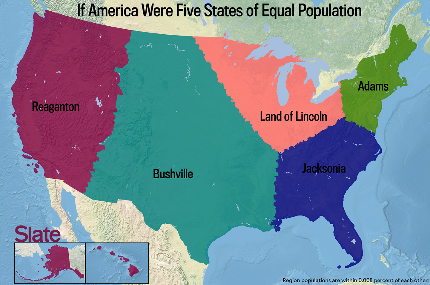
- I placed two households in each of the five areas of equal population according to a map that used Census data.[54] The 11th household was added to represent a region that I had otherwise missed (the Pacific Northwest).
- 30 percent of households are in central cities, 61 percent are in suburbs, and 9 percent in rural areas.[55]
- I chose household sizes that represented the U.S. population: 10 percent in single-member households, 26 percent in two-member households, 18 percent three-member households, 21 percent in four-member households, 12 percent in five-member households, 6 percent in six-member households, and 7 percent in households of seven or more.[56]
- 23 percent of Americans are children.[57]
Total Expenditure and Distribution
I distributed total expenditure among the 11 households to match per-capita consumption implied by the National Income and Product Accounts for 2015 Quarter II. Since the NIPA does not provide distributional information, I used several sources to create a plausible distribution across the 11 households. In the 11-household distribution, 12 percent of the population lives in a pair of households that enjoy 45 percent of total consumption. That is probably more concentrated than actual U.S. consumption and about as concentrated as U.S. income.
According to the World Top Incomes Database, the top 10 percent of tax units earn 50 percent of all income including capital gains.[58] According to CBO estimates, the top 10 percent of households (weighted by size) earn 34 percent of income. Since wealthier households save more, pay higher tax rates, and receive little of their income in transfers, consumption inequality is substantially lower than income inequality.
According to one estimate of consumption inequality, the ratio of the average consumption of the 80th to 95th percentile of households to that of the 5th to 20th percentiles is around 3.5.[59] Comparing the second and third richest households in my distribution to the bottom three households yields a similar ratio (3.6).
Another estimate of the distribution of consumption among households ranked by income found much lower inequality. The top-earning 20 percent of households enjoyed only 29 percent of total consumption, barely double the consumption of the bottom-earning 20 percent.[60] Perhaps this very equal distribution of consumption was due to retirees consuming out of their wealth?
Housing
- Homeowning households comprise 63 percent of households; renters 37 percent.[61]
- The median home value in the U.S. is about $180,000.[62]
- The user cost of housing is 6.5 percent.[63]
- I overshot the NIPA aggregate expenditure on home rental due to the inclusion of a family paying high rent in Manhattan, which is atypical, and undershot the aggregate expenditure on owner-occupied housing to compensate.
- I matched the NIPA aggregate expenditure on all housing plus an estimated 1 percent of owner-occupied home value in property taxes.
Other Expenditures
Using NIPA expenditure shares, my 11 households accurately matched aggregate expenditures on:
- Food at home,
- Food away from home,
- Electricity,
- Natural gas,
- Fuel oil,
- Auto purchase,
- Gasoline and motor oil, and
- Health care.
Visible v. Total Consumption
To allow readers to compare their perceived consumption with public consumption figures, I defined “visible consumption” to equal total consumption minus the user costs of homeowning and money spent by insurers on one’s behalf. Consumers wishing to compute their own visible consumption should subtract their annual net savings from their after-tax income and should further deduct mortgage payments, property taxes, and homeowners’ insurance. The concept is closer to what is reported by participants in the Consumer Expenditures Survey than to the NIPA measures of overall consumption.


