The “social cost of carbon” (SCC) is a metric used by the Environmental Protection Agency (EPA) to quantify the economic impact associated with carbon emissions.[1] The EPA uses three statistical models to estimate the SCC: FUND (Climate Framework for Uncertainty, Negotiation and Distribution), DICE (Dynamic Integrated Climate-Economy), and PAGE (Policy Analysis of the Greenhouse Effect).[2] Although policymakers often refer to the results generated by these models to justify imposing burdensome regulations on the energy sector of the U.S. economy, the fundamental assumptions underlying these models have a number of serious deficiencies.[3] In this study, we look at several of these shortcomings in the DICE model.

In particular, aside from the serious questions concerning the core of integrated assessment models (IAMs) in general, the DICE estimates of the SCC shift substantially with reasonable alternatives to just a few assumptions.[4] For instance, our analysis shows that:

• Using a discount rate (a measure of the time value of money) mandated by the Office of Management and Budget (OMB) that the EPA omitted reduces the 2020 estimate of SCC by more than 80 percent;
• An updated estimate of the equilibrium climate sensitivity distribution (ECS)—a measure of CO2’s temperature impact—reduces the 2020 estimate of SCC by more than 40 percent; and
• With an updated ECS distribution, a time horizon up to 2150, and with the omitted discount rate, the 2020 estimate of SCC falls by nearly 90 percent, from $37.79 to $4.03.

Originally devised by William Nordhaus in the early 1990s, the DICE model estimates the SCC based on five scenarios of economic growth projections, population growth projections, forecast CO2 emissions, and forecasts of non-CO2 forcings.[5] We recently published a comment to the Department of Energy, investigating how changes to the discount rate, time horizon, and ECS distribution affect the DICE model’s computation of the SCC under one such scenario.[6] This study represents a considerably more comprehensive analysis, averaging the results across all five scenarios.

An Overview of the DICE Model

The DICE model attempts to quantify how the atmospheric concentration of CO2 negatively affects economic output through its impact on global average surface temperature. In the model, a series of equations represents world economic activity, the CO2 levels that activity generates, and the impact of the resulting CO2 levels. Each SCC estimate is the average of numerous iterations (10,000 in the EPA’s assessment, which we reproduce here) of the model using different potential values for climate sensitivity (how much warming a doubling of CO2 will generate).[7]

For each year, the model looks at the future incomes and environmental losses for the business-as-usual case and compares it with one with higher CO2 emissions. The aggregated difference in these values determines the SCC.

Discount Rate

Economists use cost-benefit analysis to determine whether an action or rule makes economic sense. The goal is to use measures of costs and benefits closest to those of the people affected by the rule or action. The economist’s role is not to establish how much people should value items gained or lost, but to calculate based on observing how much these people actually value these items.

Because people prefer benefits sooner rather than later and costs later rather than sooner, it is necessary to adjust the values of costs and benefits when they occur at different times. For instance, few people would accept an offer of $1 per year for the next 50 years in exchange for $50 right now. There is a risk that the full $50 will not be repaid. There may be investment opportunities that will repay more than $50, and there is simply a very human preference for earlier satisfaction. Interest rates on loans and investments reflect these preferences to receive benefits now and pay costs later. Interest rates are used in the discounting process to put the costs and benefits on an equivalent time basis according to people’s observed preferences.

The interest or discount rate that economists choose is not prescriptive, but descriptive. If a 7 percent discount rate makes people indifferent between a benefit now versus a benefit later (for example, indifferent between $100 today versus $107 a year from now), then 7 percent is the appropriate discount rate to use.

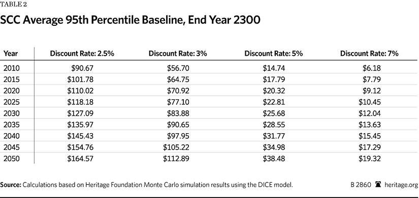
The Office of Management and Budget stipulates that government agencies should bracket their cost-benefit analyses by using discount rates of both 3 percent per year and 7 percent per year. Although there may be some flexibility to use discount rates outside these two percentages, cost-benefit estimates using other discount rates are to be in addition to the 3 percent and 7 percent estimates, not in place of them. However, the EPA has presented SCC computations based only on 2.5 percent, 3 percent, and 5 percent discount rates.[8] In Table 1, we present the results using the EPA’s 2.5 percent, 3 percent, and 5 percent discount rates as well as using a 7 percent discount rate. Although we do not believe that 2.5 percent is an appropriate rate to use, we include estimates using 2.5 percent so that our results can be fully compared to those of the EPA.

Our estimates for 2.5 percent, 3 percent, and 5 percent discount rates are in line with results that the EPA published earlier this year.[9] The introduction of a 7 percent discount rate markedly lowers the DICE model’s SCC estimates. Estimates based on this 7 percent discount rate therefore significantly weakens the EPA’s case for adding regulations to limit CO2 emissions.

Time Horizon

As discussed earlier, the DICE model operates by summing damages over an extended time horizon. Specifically, the EPA’s estimates of the SCC are based on summing damages through the year 2300. Economists have great difficulty generating forecasts decades into the future, much less centuries. Therefore, it is highly suspect for the government to claim the capacity to base policy decisions on statistical forecasts extending nearly 300 years into the future.

We re-estimated DICE’s SCC values by summing damages through 2150 instead of 2300. Although we believe that even an end year of 2150 is still too far in the future to base meaningful policy, we compared such estimates to the baseline SCC estimates. Our results for overall means and 95th percentiles averaged over all five scenarios are in Table 3 and Table 4.

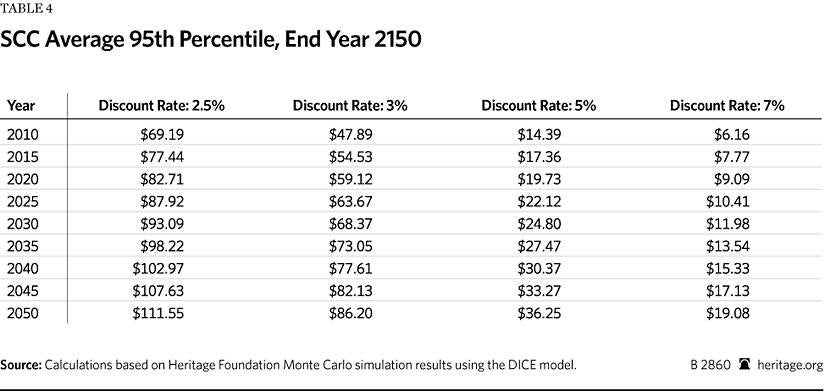
Table 5 and Table 6 and show the resulting percent changes.

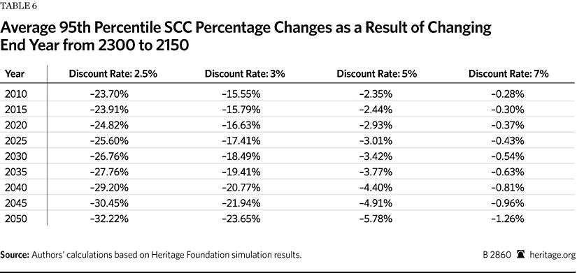
Again, we notice significantly lower estimates as a result of changing the end year.

Equilibrium Climate Sensitivity

CO2 levels are widely believed, along with many other variables, to affect the earth’s temperature. The important question is the magnitude of the impact.

As mentioned earlier, the DICE model accounts for the impact of CO2 emissions on warming by computing Monte Carlo simulations based on certain assumptions about temperature sensitivity to CO2 emissions. In particular, the model is based on an ECS distribution defined as a random variable modeling “the equilibrium global average surface warming following a doubling of CO2 concentration.”[10]

However, the EPA used an ECS distribution that was not up to date with the recent literature, creating a problem with its estimates based on the DICE model.[11] A number of recent studies offer more updated ECS distributions.[12] We chose the distribution from the Otto et al. study because it is closest distributionally to the ECS distribution assumed by the EPA in their DICE model simulations. Furthermore, almost all of the authors of the Otto study have collaborated on the Intergovernmental Panel on Climate Change’s recent “Fifth Assessment Report.”[13] Table 7 and Table 8 show our results using the Otto assumptions regarding equilibrium climate sensitivity.

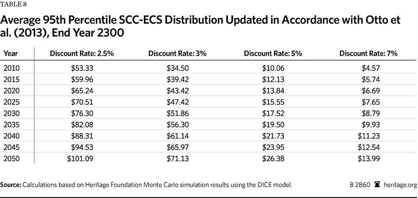
Table 9 and Table 10 show the resulting percentage changes.

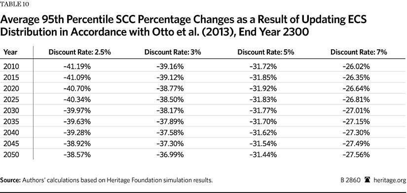
Using this more current distribution dramatically alters the SCC estimates. The ECS distribution from the Otto study is also the most conservative of the updated ECS distributions mentioned in the sense that it is closest in distribution to the Roe and Baker distribution used by the EPA. Since the other two distributions (Aldrin et al. and Lewis) are skewed even further to the left than the Otto distribution, using either of them would likely result in even lower SCC estimates.

Changing the ECS Distribution and Changing the End Year

We can amalgamate the changes in assumptions made in the previous two sections to estimate the SCC by assuming a more current ECS distribution in accordance with the Otto distribution and changing the end year to 2150. (See Table 11 and Table 12.)

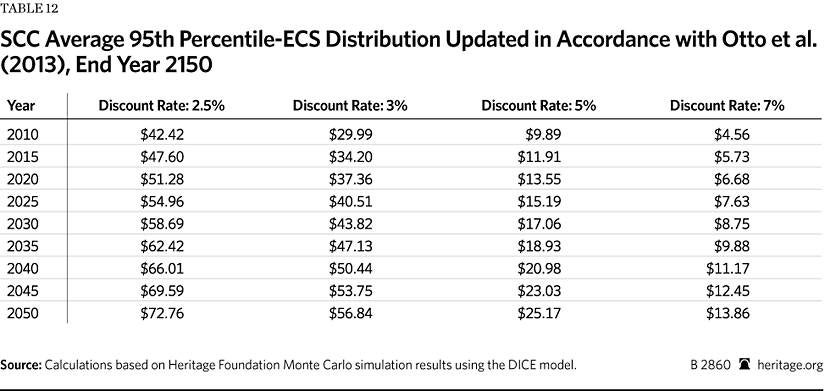
Table 13 and Table 14 show the percentage changes.

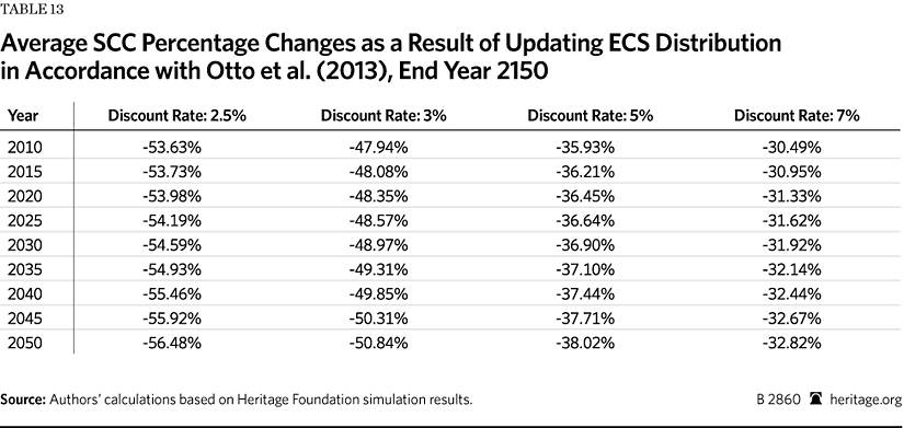
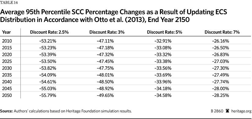
Table 14 illustrates that changing the ECS distribution in conjunction with changing the end year to 2150 results in even lower SCC estimates.

Conclusions

Our results clearly illustrate that the DICE model used by the EPA to estimate the SCC is extremely sensitive to the assumptions that we examined.

In fact, the assumptions examined in this study are not the only sensitive aspects of the DICE model. In particular, the loss functions of the DICE model and the FUND model are arbitrarily chosen, and we have yet to see sufficient justification for these functions themselves. Since the statistics estimated from these models are dependent on the model’s loss function, such justification is important because different loss functions will almost surely yield different results.

Since moderate and defensible changes in assumptions lead to such large changes in the resulting estimates of the SCC, the entire process is susceptible to political gaming. This problem exacerbates the model’s more fundamental and more serious shortcomings in estimating damages in the first place. While running the DICE model (and similar integrated assessment models) may be a useful academic exercise in anticipation of solving these very serious problems, the results at this time are nowhere near reliable enough to justify trillions of dollars of government policies and burdensome regulations.

—Kevin D. Dayaratna is Research Programmer and Policy Analyst and David W. Kreutzer, PhD, is a Research Fellow for Energy Economics and Climate Change in the Center for Data Analysis at The Heritage Foundation. The authors would like to thank Pat Michaels and Chip Knappenberger of the Cato Institute for previous discussions and assistance with this study.