A government’s budget reflects its priorities. Choices about what to tax and what to subsidize follow from legislators’ priorities about what to discourage and what to encourage. Taxes, transfer spending, and debt financing reflect distributional concerns about who should bear the costs of government and who should receive additional benefits.REF
Fiscal choices have profound effects on the economy. Households’ and firms’ choices about what to buy and sell are affected by how taxes and subsidies distort market prices. Their economic decisions are inseparable from the prevailing fiscal policy.
A plan for fiscal policy that ignores its macroeconomic effects tells an incomplete story. Legislators need the full story about how taxes and spending will affect the economy when planning a budget for the government. The agencies that produce estimates of the budgetary effects of bills for Congress, the Congressional Budget Office (CBO) and the Joint Committee on Taxation (JCT), will incorporate macroeconomic feedback in their estimates but only for major bills and only upon request. Many ideas that are a part of the larger debate about the budget are not able to receive a complete estimate because of the time and resources needed for CBO and JCT to model macroeconomic effects.
This Issue Brief produces similar estimates for the proposals in The Heritage Foundation’s Budget Blueprint for Fiscal Year 2023. The Budget Blueprint is a plan to reduce the economic distortion of taxation and bring spending in line with tax revenue. By producing a dynamic score of the Blueprint, Heritage hopes to add new information to the debate as legislators consider bills with fiscal effects.
The results presented here use a computable general equilibrium (CGE) model under development within Heritage’s Center for Data Analysis. In this CGE model, households, firms, and governments participate in markets. Households and firms trade to maximize utility and profit, respectively. Their supply and demand curves are the solutions to forward-looking optimization problems, which means they respond to current and future changes in policy. Government policy, such as the current law baseline or the Budget Blueprint, is an input into the model. The model’s output is a solution for wages and interest rates that clear markets in equilibrium along a balanced growth path. More details and a brief description of the solution procedure are presented at the end of this Issue Brief.
Economic Principles to Create a Larger Economy
The goal for fiscal policy should be to maximize gains from trade, letting as many people improve their lives as possible. A market without taxes achieves this goal, reaching an equilibrium when the cost to produce a good equals the value of the good to the consumer.
Taxes distort economic decisions. Households and firms try to reduce the cost of taxes by buying or producing less of a taxed good. The tax creates a wedge between the price paid by a consumer and the price received by a producer. Any trade that does not produce surplus value greater than the tax wedge never occurs. Thus, the costs from taxation for society include not just the tax revenue paid to the government but foregone value from trades that never occur.
Keeping taxes low reduces economic distortion. Some level of taxation is unavoidably necessary, but ideally the government would raise revenue in the least distorting way by collecting small rates on a large base.
When there is more trade because of lower taxes, there is a bigger tax base for the government to raise revenue. For example, the Blueprint proposes adopting neutral cost recovery for structures and reducing the corporate income tax rate as specific taxes that should be reduced. The reduction of taxes on capital are responsible for most of the increase in output. Lower tax rates start a chain of cascading economic developments:
- Lower taxes on capital income increase the returns to saving and investment.
- Firms want to invest more and households are willing to save to finance the investment.
- With the additional capital, firms produce more goods and services.
- Households incomes increase as the value of what capital and labor produce increase.
- Consumption increases as more goods and services are produced.
- Federal tax revenues increase, because revenue is proportional to incomes and production.
Effects in the 10-Year Budget Window
Table 1 shows revenues, outlays, surpluses, debt, and gross domestic product (GDP) under model equivalentsREF of the CBO baseline and the Blueprint’s proposals. The static estimate is calculated by applying the proposed policies to economic tax bases from the baseline. The dynamic estimate allows labor and capital markets to find a new equilibrium and calculates budget figures using the updated bases. Using model equivalents puts the different estimates on equal terms, allowing an apples-to-apples comparison of the static and dynamic effects, which are reported in the bottom half of Table 1.
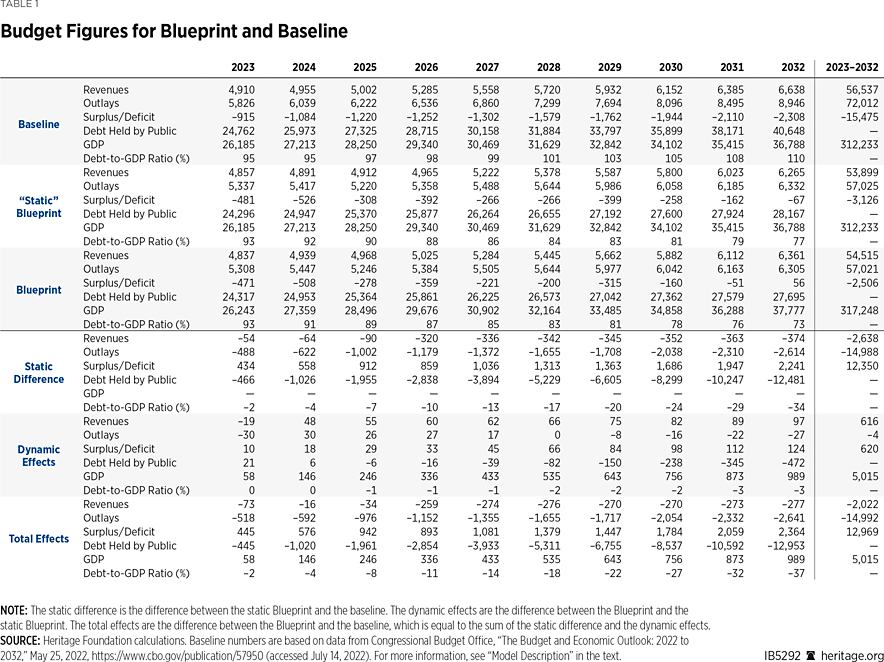
The reduction in tax rates provides incentives for households to work and firms to invest. The reduction in income tax raises after-tax wages, leading to an increase in hours worked. After-tax wages increase by 3.5 percent and hours worked increase by 4.2 percent at the end of the 10-year budget window. For reference, that is equivalent to $2,200 for the median household and 6.0 million full-time equivalent jobs.REF Additional investment increases the capital stock by 2.9 percent after 10 years. The additional labor and capital results in increased GDP. At the end of the 10-year budget window, GDP is 2.7 percent higher than in the baseline.
The increase in GDP raises projected revenues relative to traditional estimates. As economic activity increases, the government takes a smaller share of a bigger pie. While macroeconomic effects indicate that revenue would be higher than what a traditional estimate would suggest, the net result of lower tax rates is a reduction in revenue.
Over the 10-year window, the increase in revenue from dynamic effects is about 23 percent of the static reduction. The relatively small effect in the budget window is because dynamic effects operate through capital accumulation, which occurs over time and continues outside the budget window. Over the first 25 years, dynamic effects recover about 39 percent of the static cut. The dynamic effects on revenues are in line with general estimates reported elsewhere in the literature.">REF
The increase in GDP is due to increased activity in financial markets. Under the Blueprint, reduced tax rates mean that firms increase investment and look to borrow more to finance it. For a given amount of savings from households, when more of it is used to finance private investment, there is less available for the government to finance its budget deficit. Thus, the government must pay higher interest rates to secure a share of the more limited funding.
The Blueprint reverses the standard story about crowding out in financial markets. The standard story to illustrate crowding out considers an increase in government spending financed by issuing new debt. For a given amount of savings from households, when more of it is used to purchase government debt, there is less available for firms to finance investment in capital. Firms with particularly productive investment projects bid up interest rates to secure a share of the more limited funding.
Therefore, macroeconomic effects raise outlays relative to a traditional estimate. While the Budget Blueprint would significantly reduce total outlays using both traditional and dynamic estimates, the reduction in outlays is less when incorporating the macroeconomic effects because of increased interest rates on federal debt. This insight highlights the importance of understanding why prices change. Though the increase in interest raises interest costs for the federal government, it is worth the benefits of increased investment.
Under both the static and dynamic estimates of the Blueprint, debt held by the public falls relative to GDP. While debt held by the public in 2032 is about $40 trillion in the baseline, it is about $28 trillion under the Blueprint. The debt falls primarily because large reductions in outlays reduce the deficit relative to the baseline.
Accounting for dynamic effects reduces the estimate of the debt in 2032 by about $475 billion. The additional reduction and debt and the increase in GDP imply that the ratio of debt to GDP falls to 73 percent instead of 77 percent.
The Budget Blueprint Produces Long-Lasting Growth
A key feature of the model is adjustment costs when firms change the capital stock. Adjustment costs are needed for the model to match data regarding the pace of investment in response to policy changes. As a result, capital accumulates slowly over time as firms build up toward the higher equilibrium capital stock. Revenues grow over time as firms invest in capital and increase output.
Indeed, the beneficial effects of the Blueprint’s policies continue well after the 10-year budget window. Adjustment costs mean that the capital stock takes many years to converge to the new equilibrium growth path, raising growth rates well into the future. Due to the increases in investment and labor, real GDP growth is elevated by at least 0.20 percent per year for the first 10 years, by at least 0.10 percent per year for the first 17 years, and by at least 0.05 percent per year for the first 33 years.
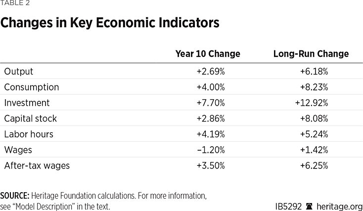
In the new equilibrium, GDP is 6.18 percent higher than in the baseline. Much of the increase occurs outside the 10-year budget window. Consumption, investment, capital, labor, and wages are all higher in the long-run equilibrium than at the tenth year. The 4.00 percent increase in consumption corresponds to $678 billion per year, or $5,300 per year per household.REF The 5.24 percent increase in hours corresponds to 7.2 million full-time equivalent jobs with the current population.REF
A Bigger Economy in the Big Picture
The model used to produce these estimates is substantially simpler than what the CBO uses to produce its baseline and score legislation.REF Heritage’s model is based on a neoclassical growth model with additional detail added to capture relevant aspects for reporting budget figures. The results are presented in a format familiar to legislators that is easily compared to CBO’s estimates.
Lawmakers should keep the key insights of the model in mind when considering fiscal legislation, including appropriations bills, for FY2023. Cuts in tax rates and adjustments to the tax base will produce long-lasting economic growth. Macroeconomic effects raise revenue through higher output but not enough so that tax cuts pay for themselves. Tax cuts should be paired with spending cuts. Major spending cuts can put debt on a sustainable path.
Parker Sheppard, PhD, is Acting Director of the Center for Data Analysis at The Heritage Foundation.
Appendix: Model Description
The model used to produce these estimates has only minor changes from the model used for the FY2022 estimates earlier this year.REF The updated model includes additional detail for smaller budget line items and for converting figures in the National Income and Product Accounts to match definitions in the federal budget. The baseline was updated to reflect the most recent CBO publication in May.REF The following paragraphs reproduce the model description printed in the dynamic estimates of the FY2022 Blueprint with additional exposition for clarity.
The economic model used in this paper is a computable general equilibrium (CGE) model developed with reference to Zodorow and Diamond (2013)">REF and Heer and Maussner (2009).REF The references are handbook and textbook examples for the general class of CGE model, which is standard for showing how economies react to changes in policy.
The model has a single representative household with utility that depends on consumption of a single composite good and leisure. The representative household spends on the consumption good, purchases of equity stakes in firms, and purchases of debt issued by governments. Its income comes from providing labor to firms and governments at market wages, receiving dividends from firms’ earnings, receiving interest from government debt, and receiving transfer payments from governments. Given its budget, the household chooses consumption, labor hours, purchases of equity, and purchases of debt in order to maximize its lifetime utility.
There are two types of firms: corporate and non-corporate. Firms choose to hire labor and choose an investment plan to maximize the value of the firm to existing shareholders. Firms are assumed to pay a constant fraction of their earnings as dividends. They issue equity to cover the cost of investment above and beyond retained earnings. Additionally, corporate firms are subject to the corporate tax rate, while non-corporate firms are not.
In order to change the capital stock, firms must face adjustment costs through forgone output (such as needing to shut down a factory in order to install upgraded machinery). The presence of adjustment costs means that firms make changes to the capital stock more slowly than if adjustment costs were absent.
There are two governments in the model: the federal government and the combined state and local governments. Both governments raise revenue by levying seven types of taxes: taxes on wages, capital gains, dividends, interest, and corporate income plus payroll taxes for social benefits, and sales taxes on produced output. They spend money on purchases of the consumption good and lump-sum transfer payments to households. Value added by the governments is assumed to be a constant proportion of spending on the consumption good by governments, which raises real output, all else equal.
The model treats marginal and average tax rates separately. Marginal rates are taken directly from policy or taken as a dollar-weighted average of marginal rates when taxes have graduated brackets. Average tax rates are calibrated so that the model matches observed revenues relative to output when applied to tax bases calculated from the model.
The model is solved using the extended path method of Fair and Taylor (1983).REF Agents are presumed to have perfect foresight over future policy. They solve for the equilibrium variables over a transition path ending at the long-run steady state. The estimates presented here consider a transition path of 150 years at an annual frequency.
The federal government must have a stable debt-to-output ratio in the long-run equilibrium. Since the proposed 10-year budget plans do not produce the necessary surpluses, nor does current law within the next 30 years, the model presumes that efforts to stabilize the debt start after 30 years. The government sets a target debt-to-output ratio and reduces the excess debt by 1 percent per year by reducing transfer payments to households.


