SECTION 1: INTRODUCTION AND SUMMARY
Changes in tax policy can influence economic incentives for households to work and save and for businesses to invest. Subsequent changes in employment, investment, and incomes can affect federal tax revenues. Dynamic analyses capturing such interactions between taxes and the economy are facilitated by integrating macroeconomic models of the economy and microsimulation models of taxation. An important part of that integration is calibrating both models to the same "baseline" forecast.
In this paper, we describe a process for calibrating a macroeconomic model of the U.S. economy and a microsimulation model of the federal individual income tax to the Congressional Budget Office's (CBO's) January 2006 baseline projections. The microsimulation model is based on the Public Use Tax File produced by the Statistics of Income (SOI) Division of the Internal Revenue Service (IRS). The macroeconomic model, Global Insight's U.S. Macroeconomic Model, is based on Bureau of Economic Analysis (BEA) national income and product accounts (NIPA) data.[1] Once calibrated to the same official baseline, the two models can be used jointly to simulate the economic and budgetary effects of changes in tax policies. Direct comparisons can then be made between dynamic estimates from the macroeconomic model and conventional estimates from the microsimulation model.
The Congressional Budget Office (CBO) produces biannual baseline projections of the U.S. economy and the federal budget (generally in January and August of each year). Those projections embody the rules and conventions governing a current-services federal budget. They project gross domestic product (GDP), prices, personal and corporate incomes, and federal receipts, expenditures, and net saving, among other economic and budgetary variables over 10 years assuming current-law tax (and non-tax) policies and the continuation of current levels of spending.
CBO's 10-year baseline projections serve as Congress's official starting point for gauging the budgetary effects of proposed changes in taxes and spending. For example, the Joint Committee on Taxation (JCT) estimates the conventional revenue effects of tax proposals using CBO's economic and budgetary projections as a baseline. JCT's conventional revenue estimates may include some microeconomic behavioral effects of a change in tax policy. Thus, they may take into account shifts in the timing of transactions and income recognition.[2] But they generally exclude the economy-wide macroeconomic effects of changes in tax policy on federal receipts. Similarly, CBO uses its own economic and budgetary projections as a baseline when generating conventional estimates of the budgetary effects of spending proposals.
Simulation models meant to generate comparable "dynamic" estimates of the economic and budgetary effects of federal tax and spending proposals should also be calibrated to CBO's baseline projections. Dynamic estimates include the effects of changes in labor force participation, investment, and interest rates on federal tax policies. They can differ, sometimes significantly, from conventional revenue estimates. Dynamic estimates that are not made relative to the CBO baseline can provide a broad-brush analysis of a proposed tax policy's economic and budgetary effects. But they cannot be used as a dynamic alternative to a conventional estimate of the proposed policy's effects. At best, they can serve as a vehicle for ranking the relative strengths and weaknesses of alternative proposals.[3]
We calibrate two models to CBO's baseline economic and budgetary projections. We typically use both models to evaluate proposed changes in tax policy. The first model is the Global Insight (GI) short-term U.S. Macroeconomic Model. The second is a proprietary microsimulation model of individual income tax returns developed by analysts at The Heritage Foundation's Center for Data Analysis.
A CBO-like baseline forecast is constructed using the Global Insight model and the details that CBO provides about its economic and budgetary projections. Using the GI model, we infer the implications of CBO's current-law assumptions for key macroeconomic variables, including personal consumption, investment, employment, and the components of NIPA personal income. In combination with SOI data, the microsimulation model uses the final CBO-like baseline forecast and estimated relationships between NIPA personal income and personal income reported to the IRS to project the characteristics of individual income tax records. The result is an integrated calibration of macroeconomic and microsimulation models that can be used for policy simulations.
The paper proceeds as follows. Section 2 gives key facts about CBO's baseline economic and budgetary projections. We focus on CBO's current-law assumptions and the variables CBO publishes, and we use, in calibrating to CBO's baseline projections. Section 3 discusses our general approach to calibrating the GI and microsimulation models to CBO's published projections. Section 4 concludes by examining the implications of using the calibrated macroeconomic and microsimulation models for tax policy analysis. A separate appendix considers the implications of CBO's baseline projections for key measures of macroeconomic activity and incomes.
SECTION 2: AN OVERVIEW OF CBO'S BASELINE PROJECTIONS
CBO's biannual baseline projections play a dual policy role. They inform policymakers about the implications of current fiscal policies for federal budgetary aggregates, and they provide a common baseline for scoring the budgetary effects of proposed changes in taxes and spending. As a result, CBO's economic and budgetary projections are unique when compared with other -- particularly commercial -- forecasts. Specifically, they embody current law, and they explicitly assess the impact of current-law policies (fiscal and non-fiscal) on key indicators of economic activity.
CBO's Current-Policy Assumptions
A set of detailed rules govern the process by which CBO's economic and budgetary projections embody current law and policy. The Balanced Budget and Emergency Deficit Control Act of 1985 and various other conventions for a federal baseline require CBO to produce a very specific kind of forecast.[4] CBO's baseline budgetary projections -- and, hence, the CBO-like forecast we construct to replicate them -- cannot anticipate changes in current law. Rather, they must assume that future taxes, spending, and other (non-fiscal) policy measures evolve as stipulated by previously enacted legislation.
This means that CBO's 10-year revenue projections assume no change in tax provisions or tax rates unless such a change is already included in current law. Thus, CBO's January 2006 baseline revenue projections assume the 2008 expiration (or "sunset") of the preferential capital gains and dividend tax rates enacted under the Jobs and Growth Tax Relief Reconciliation Act (JGTRRA)[5] and the 2010 expiration of tax relief provisions enacted under the Economic Growth and Tax Relief Reconciliation Act (EGTRRA).[6] Similarly, despite widespread discussion of the issue, CBO's revenue projections do not include any changes to the alternative minimum tax (AMT). Private sector forecasts typically anticipate some change in the current law governing the AMT -- if only because without some adjustment a growing number of taxpayers will see their tax burdens increase as a result of the AMT.
CBO's budgetary projections also exclude changes in federal spending not already set by current policies. Thus, CBO uses current-law eligibility and benefits criteria to project mandatory spending on entitlement programs like Social Security, Medicare, and Medicaid over the 10-year budget period.[7] Current law in the form of appropriations bills does not dictate a path for discretionary spending and supplemental budget authority beyond the current budget year.[8] However, the Balanced Budget and Emergency Deficit Control Act of 1985 requires that CBO assume that both discretionary spending and supplemental appropriations in the most recent year's budget authority continue in each subsequent year of CBO's 10-year budgetary baseline.[9] In that baseline, projected current-services outlays keep pace with projected current-services budget authority. Both projected budget authority and outlays rise because CBO adjusts budget authority to offset projected inflation and cost-of-living adjustments.
CBO assesses the impact of GDP, prices, interest rates, incomes, and other economic variables on current-law revenues and spending over a 10-year period. CBO's baseline economic projections consist of two conceptually and analytically distinct components -- a two-year (short-term) forecast of cyclical fluctuations and a separate eight-year (medium-term) projection of potential output (GDP).[10] This split in the budget period determines how CBO assesses the economic implications of current-law fiscal policies.
In the short term, CBO allows the path of GDP to deviate from that of its underlying potential.[11] CBO gauges the impact of the gap between actual and potential GDP on a range of economic variables. Those variables include inflation, interest rates, employment, personal and corporate incomes, personal consumption and saving, and residential and business fixed investment. CBO also anticipates how monetary policy, exchange rates, and energy prices as well as recently enacted changes in current-law policies (fiscal and non-fiscal) are likely to affect fluctuations in aggregate demand. For example, the August update to CBO's January 2003 The Budget and Economic Outlook estimated the impact of JGTRRA's partial-expensing provisions on business fixed investment in 2003 and 2004.[12] It also discussed the effects of JGTRRA's accelerated tax cuts on personal saving.[13]
In the medium term, CBO does not project fluctuations in aggregate demand. Instead, it uses a growth model to estimate potential GDP and assumes that any gap between actual GDP and estimated potential GDP remaining at the end of the short-term forecast closes over the subsequent eight years.[14] Other key economic variables are similarly assumed to trend toward an estimated long-run average over the medium term. For example, CBO's projected rate of return on 10-year Treasury notes equals 5.2 percent from 2007, one-year prior to the start of CBO's medium-term projections.[15] CBO's projected unemployment rate attains its long-run natural rate (5.2 percent) only two years later, in 2009. In contrast, the unemployment rate in Global Insight's February 2006 short-term U.S. Macroeconomic forecast fluctuates around its long-run natural rate over much of GI's 10-year forecast horizon.[16]
As a result, CBO's medium-term projections are largely limited to assessing the impacts of current-law fiscal policies on potential GDP and related variables, notably potential labor hours and capital. For example, EGTRRA's expiring provisions and increasing taxpayer exposure to the AMT are likely to generate a steady rise in average marginal tax rates on wages. CBO adjusts potential labor hours for the anticipated disincentive effects, layering an estimated decline in the supply of labor hours onto a baseline projection that reflects long-run trends in demographics and labor force participation.[17] CBO also estimates the potential effects of rising federal deficits and debt on the capital stock. It includes some "crowding out" of private investment into its growth model, using projections of net foreign investment to gauge the extent to which increased capital inflows from abroad are likely to offset declines in national saving and domestic private investment.[18]
Federal Policy Assumptions Found in Other Macroeconomic Forecasts
Unlike CBO, other forecasters -- particularly commercial forecasters -- are not restricted by the rules and conventions governing a federal baseline. They can therefore build into their forecasts expected changes in taxes and spending that are inconsistent with a current-law baseline. They can also anticipate changes in other, non-fiscal current-law policies. Those expectations about future fiscal and non-fiscal policies can dramatically impact projected values of key economic and budgetary aggregates.
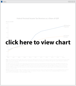
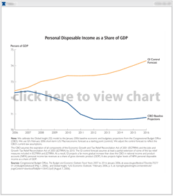
For example, GI's February 2006 U.S. Macroeconomic forecast assumes a partial extension of expiring tax relief provisions originally enacted under EGTRRA and JGTRRA. As a result, GI projects a far more gradual increase than does CBO in NIPA personal income tax revenues as a share of GDP (see Figure 1A). Unsurprisingly, GI also projects higher levels of NIPA personal disposable income as a share of GDP -- particularly after 2010 (see Figure 1B).
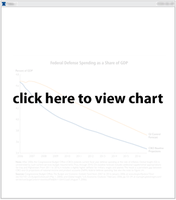
Commercial forecasts can also include expected changes in federal spending that are inconsistent with a current-services budget.[19] Both CBO's baseline budgetary projections and GI's February 2006 U.S. Macroeconomic forecast allow for growth in federal defense spending over the next 10 years. However, GI consistently projects higher levels of defense spending as a share of GDP (see Figure 2).
Initial differences between CBO's and GI's projections of defense spending seem in part explained by different assumptions about the rate of spending. Federal defense spending fell in the fourth quarter of 2005, after expanding at a double-digit rate in the third quarter of the same year.[20] It followed a similar pattern in the final two quarters of 2004 before bouncing back strongly in the first quarter of 2005. GI largely attributes both third-to-fourth quarter declines to delays in the passage of the current fiscal years' defense appropriations bill.[21] Using history as a guide, it assumes a strong rebound in defense spending in the first half of 2006. Such a strong rebound in federal defense spending is not as apparent in CBO's budgetary projections.[22]
After 2006, CBO projects current fiscal-year defense spending forward at the rate of inflation. GI is not restricted by such current-services budget requirements. Thus, through 2010, GI's standard forecast includes additional supplemental appropriations for Iraq and Afghanistan. From 2011 to 2016, it includes a slightly higher deflator for military wages and salaries. The result is a persistent gap between CBO and GI projections of NIPA federal defense spending.[23]
Finally, commercial forecasts can anticipate changes in other (non-fiscal) current-law policies. The Pension Funding Equity Act of 2004 (PFEA) expired at the end of 2005. PFEA temporarily lowered firms' required contributions to defined-benefit (DB) pension plans. It did so by setting the maximum applicable discount rate used to calculate the present value of DB pension liabilities above the rate required by the Employment Retirement Income Security Act of 1974 (ERISA). In general, the higher the applicable discount rate, the lower the present value of pension liabilities and the lower required DB pension contributions.[24]
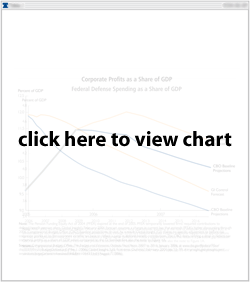
GI's February 2006 U.S. Macroeconomic forecast assumes a change in current law that extends PFEA's higher discounting through 2006. CBO's baseline economic and budgetary projections do not.[25] As a result, GI makes no specific adjustments to corporate (book) profits or to the corporate income tax base to reflect a jump in DB contributions. CBO includes such adjustments, dramatically lowering projected corporate profits as a share of GDP relative to the GI forecast (see Figure 3).
Limitations of Using CBO's Published Baseline Projections
We calibrate a commercial macroeconomic model of the U.S. economy and a proprietary microsimulation model of individual income tax returns to CBO's baseline projections. The challenges faced in calibrating the two models differ. However, for both models, a common factor complicates our work. CBO publishes only a small subset of the economic and budgetary variables making up its baseline projections (see Table 1). This limits the number of variables available as guides in adjusting the two models to reflect CBO's current-law assumptions.
Calibrating the Global Insight Model. We develop our CBO-like baseline forecast using GI's February 2006 U.S. Macroeconomic forecast as a starting point (or control).[26] GI's U.S. Macroeconomic forecasts typically include expected changes in fiscal and non-fiscal policies. The calibration procedure in part involves iteratively adjusting the control forecast to remove the effects of those expectations so that our CBO-like forecast is consistent with current law.
Adjusting the control forecast to match CBO's baseline budgetary projections is relatively straightforward. CBO publishes all but a handful of needed NIPA federal revenue and spending projections. It also provides a detailed crosswalk between its NIPA federal budget numbers and its projections of unified (budget) federal revenues and unified federal outlays.[27]
However, CBO does not publish its projections of a number of key macroeconomic and income variables. Those variables include the components of GDP, NIPA taxable personal income (with the exception of wage and salary income), and national saving (with the exception of NIPA net federal government saving).[28] They also include a number of miscellaneous items describing critical assumptions (policy and otherwise) underlying CBO's two-year forecast and medium-term projections.
For example, CBO does not typically describe in great detail its projections of the trade-weighted U.S. dollar exchange rate, the price of oil, and the federal funds rate. Rather, the economic outlook chapter of The Budget and Economic Outlook indicates CBO's expectations for their levels or movements in the short term.[29] When calibrating the GI model to CBO's baseline economic projections, we use such statements as guides in adjusting (if necessary) GI's projections of equivalent variables.
Thus, in August 2005, CBO indicated that it expected oil prices to stop rising -- but not to "retreat" to pre-2004 levels -- during 2005 and 2006.[30] In January 2006, CBO again indicated that it expected oil prices to stabilize in 2006.[31] We adjusted a weighted average price of imported crude in the GI model appropriately. Similarly, in August 2005, CBO anticipated that the Federal Reserve would continue to raise the target for the federal funds rate until it reached a neutral rate. CBO observed that the consensus of financial market participants was consistent with a neutral rate ranging between 4 and 5 percent.[32] In January 2006, CBO reconfirmed its outlook for monetary policy, specifying that the consensus of financial market participants put the expected federal funds target rate at 4.75 percent by mid-2006.[33]
More significantly, CBO does not typically provide sufficient detail to establish how it adjusts a number of key macroeconomic and income variables to reflect current law. Figures 4 and 5 reorganize NIPA data as a series of income and expenditure flows among institutional sectors of the economy (households, firms, government, rest of the world, etc.).[34] Moving across the columns gives an accounting of income flows among the sectors. Moving down the rows gives an accounting of expenditure flows.
Figure 4 broadly summarizes the level of detail we require for calibration of the microsimulation model and for policy analysis. For example, calibrating the microsimulation model to CBO's baseline budgetary projections of individual income tax receipts requires projections of the individual components of NIPA personal income.[35] Calculating the federal corporate income tax requires projections of both corporate profits and the corporate income tax base. Finally, doing dynamic analyses of fiscal policy requires the ability to quantify the effect of changes in taxes and spending on the components of GDP and personal income.
The Global Insight model, once calibrated to CBO's published baseline projections, provides this level of detail. A forecasting model like Global Insight provides unique advantages to analysts constructing a CBO-like baseline forecast. This is because it includes enough structural detail to fill in the blanks left by CBO. Figure 5 highlights the extent of those blanks. It shows the same reorganization of NIPA income and expenditure flows as Figure 4, but with identifiers only in the cells for which CBO publishes its baseline economic projections. We use the GI model to help us infer consistent approximations of CBO's projections of the missing income and expenditure flows (see Appendix A for additional details).
CBO's current-law assumptions complicate our efforts to infer those projections using the GI model. For example, the control forecast implicitly assumes some extension of EGTRRA's expiring provisions after 2010. It therefore includes levels of personal consumption and saving that are higher than those projected by CBO. The calibration procedure involves iteratively lowering the projected rate of growth in personal consumption implied by the control forecast so that the projected personal saving rate is not unreasonable. Unfortunately, CBO typically provides little or no detail on how it adjusts consumption and saving to reflect EGTRRA's sunset. As a result, we have only personal judgment and historical data to rely upon when determining an appropriate current-law level for the personal saving rate.
Similarly, CBO typically publishes only its projections of NIPA taxable personal income and wage and salary income.[36] Calibration requires allocating the difference between the two among personal dividend income, personal interest income, personal rental income, and proprietors' income (farm and non-farm). We can use information from the control forecast to do this. However, the control forecast implicitly assumes some extension of JGTRRA's preferential tax rates on dividend income. And CBO typically provides little or no additional detail to use in deriving an allocation that would be more consistent with current-law assumptions.
Calibrating the Microsimulation Model. The primary challenge we face in calibrating the microsimulation model to CBO's baseline projections is a bit different. The inputs into the calibration procedure for the microsimulation model already reflect current law. For example, we use a number of economic variables from the CBO-like forecast. We also use many of the federal revenue projections published in the revenue outlook chapter of CBO's The Budget and Economic Outlook.
However, economic inputs from the CBO-like forecast provide only a starting point. This is because they are expressed as NIPA values and not as amounts reported on tax returns. The microsimulation model simulates the effects of tax law changes on a representative sample of over 100,000 federal individual income tax returns based on the characteristics of the individuals and families associated with those returns. A crosswalk is therefore needed to reconcile the definitional and timing differences between NIPA personal income, the amount of income reported on income tax returns, and supplementary information obtained from the Current Population Survey (CPS). Non-NIPA components of individual income such as capital gains, pensions, annuities, and individual retirement accounts must also be added. Data for tax return filers and non-filers must then be extrapolated ("aged") over the 10-year budget period.
As a result, a key part of our calibration procedure involves deriving detailed targets for the amount of tax-related income, the distribution of tax-related income, and the demographic characteristics of the U.S. population. These targets are then used to adjust data on records in the microsimulation model so that those records are in aggregate consistent with CBO's baseline economic and budgetary projections. Such information is not typically published by CBO and cannot generally be obtained directly from CBO or other sources. The exceptions are demographic projections, which are available from the Census Bureau, and projections of total individual capital gains realizations, which CBO publishes every January in The Budget and Economic Outlook.[37]
SECTION 3: CALIBRATING MACRO-ECONOMIC AND MICROSIMULATION MODELS TO CBO'S BASELINE PROJECTIONS
Calibration to CBO's baseline projections begins with the macroeconomic model. We first calibrate the Global Insight model to CBO's published economic projections and NIPA federal revenue and spending projections. We refer to output from the calibrated GI model as the final CBO-like forecast. The final CBO-like baseline forecast not only replicates the published details of CBO's current-law baseline but also includes projections of key macroeconomic and income variables excluded from them (see Appendix A for additional details).
We then calibrate the microsimulation model to CBO's baseline projections. In doing so, we use data from the SOI and the Census Bureau as well as economic variables from the final CBO-like forecast. Those economic variables include nominal GDP, corporate profits, the consumer price index (CPI) for all urban consumers, the components of NIPA taxable personal income, NIPA transfer payments to persons (federal as well as state and local), and NIPA state and local tax revenues. The calibrated microsimulation model that results approximates CBO's baseline projections of key economic and income variables and individual income tax revenues.
Calibrating the Global Insight Macroeconomic Model
Calibrating the Global Insight model to CBO's current-law baseline involves iteratively adjusting the control forecast so that, when solved, the Global Insight model endogenously reproduces all projections of economic and budgetary variables published by CBO.[38] This is a multi-step process. In each step, we replace variables in the GI model with CBO's projections. We then solve the GI model so that those variables that have not been targeted adjust. In essence, we are using econometrically estimated relationships and accounting identities within the GI model to create a forecast that is consistent with what we know about CBO's baseline economic and budgetary projections.
Step 1. We first set key economic assumptions and price levels. This process involves setting the price of oil and the trade-weighted U.S. dollar exchange rate so that they are consistent with what we know about CBO's baseline economic assumptions. It also involves setting some policy variables such as the statutory corporate income tax rate and the federal social insurance tax rate so that they are consistent with CBO's baseline revenue projections. Finally, it requires that we impose CBO's projections of certain key economic variables. Those variables include the unemployment rate, the 3-month Treasury bill rate, and the 10-year Treasury note rate.
The 3-month Treasury bill rate is also used to set the federal funds rate. The GI control forecast includes a projection of the federal funds rate that differs from what CBO describes as the consensus of financial market participants. We correct for this by imposing a target for the federal funds rate that is broadly consistent with not only CBO's description of financial market consensus but also CBO's projection of the 3-month Treasury bill rate. We obtain this target by first calculating the spread in the control forecast between the 3-month Treasury bill rate and the federal funds rate. We then apply this spread, with some adjustments, to CBO's projection of the 3-month Treasury bill rate.
We complete the first step by setting price levels for all components of GDP. CBO publishes 10-year projections of year-over-year percentage changes in an aggregate GDP price index. We use this along with information about the components of the GDP price deflator contained in the GI control forecast to set all underlying GDP price indices so that they are consistent with CBO's projection of GDP inflation.
Setting price levels early in the calibration procedure is critical. This is because many exogenous federal outlays variables in the Global Insight model are in real (inflation-adjusted) terms. We therefore require a price level variable to convert CBO's nominal baseline budgetary projections for those variables into consistent real targets.
Step 2. In the second step, we set federal spending (outlays) net of federal interest payments.[39] Federal spending broadly includes federal consumption spending, federal transfer payments, and other spending items in the federal government's budget.
CBO publishes its projections for most -- but not all -- of the Global Insight model's NIPA federal spending variables. For example, the federal government's budget includes federal social benefits to the rest of the world and federal subsidies. CBO publishes its projections of both aggregates. We replace GI's projections of these variables with CBO's published NIPA projections. Similarly, CBO publishes its projection of federal net investment.[40] We combine this with CBO's baseline projections of NIPA defense and non-defense consumption of fixed capital to obtain a NIPA target for federal gross investment.
However, CBO does not provide baseline projections for all NIPA federal spending variables. In some instances, we rely upon the GI control forecast to obtain needed targets. For example, federal consumption spending includes both defense and non-defense "other" purchases of goods and services and wages and salaries for personnel. CBO only publishes its projection of the sum of the two (labeled defense and non-defense "consumption"). In the absence of any additional information from CBO, we set "other" federal purchases of goods and services equal to the difference between CBO's projections of defense and non-defense "consumption" and GI's projections of defense and non-defense outlays for personnel.
In other instances, we derive needed targets from CBO's published projections of budget (unified) federal outlays. Federal transfer payments include both social benefits to persons and grants-in-aid to state and local governments. CBO publishes its NIPA projection of grants-in-aid to state and local governments. However, it publishes only budget projections of federal spending on Social Security, Medicare, and Medicaid. To obtain equivalent NIPA targets, we use historical government social benefits data from CBO and BEA to adjust CBO's published projections of Social Security, Medicare, and Medicaid spending for administrative costs.[41]
Step 3. In the third step, we adjust the components of GDP so that they are consistent with not only CBO's projections of real GDP and real federal spending (on both current consumption and investment) but also current laws and policies. We follow a three-step procedure.
First, we adjust all components of GDP for which CBO's baseline projections are unavailable. Those components include personal consumption, gross private domestic investment, state and local government purchases of goods and services (including state and local investment), and net exports. We scale all four aggregates proportionately so that they are consistent with CBO's projections of real GDP and real federal spending. We do so using information from the control forecast about the allocation of GDP among its constituent components.
Second, we derive a target for personal consumption that is more in line with CBO's current-law assumptions. A target for real personal consumption obtained using information strictly from the control forecast is likely to be too high. This is because the control forecast does not assume current law. CBO does not describe in detail its baseline projections of personal consumption. However, the economic outlook chapter of The Budget and Economic Outlook typically gives annual rates of growth in personal consumption for the two years covered by CBO's short-term economic forecast.[42] We derive a target for real personal consumption using those growth rates and some judgment about the likely impacts on personal saving of not extending EGTRRA's and JGTRRA's expiring provisions after 2010.
Finally, we readjust all components of GDP for which we do not have published projections from CBO. At this stage, those components include gross private domestic investment, state and local government purchases of goods and services, and net exports. We scale all three aggregates proportionally so that they are jointly consistent with CBO's projections of real GDP and real federal spending and our target of real personal consumption. In doing so, we again rely primarily upon information from the control forecast.
Before continuing to step 4, we consider state and local government operating surpluses in our CBO-like forecast. At this point in the calibration, state and local government purchases of goods and services, when combined with all other state and local spending, could exceed state and local revenues by a wide margin (or vice versa). CBO does not typically describe in any great detail its baseline projections for state and local government budgets. However, we assume that those budgets are roughly in balance. We adjust components of state and local spending (other than purchases of goods and services) to put state and local budgets as close as possible to a slight surplus position in the final CBO-like baseline forecast.
Step 4. We next adjust potential (full-employment) GDP in the GI model to be consistent with CBO's medium-term projections of the rates of growth in potential GDP and the potential labor force.[43]
We use the GI control forecast as a starting point. CBO does not regularly publish levels-estimates of either potential GDP or the potential labor force.[44] We therefore adjust the projected levels of both variables in the control forecast to be consistent with CBO's published growth rate projections. We apply CBO's projections of the growth rate of the potential labor force directly, adjusting the projected level of the potential labor force in the control forecast. We target the growth rate of potential GDP only indirectly, adjusting among other variables the exogenous trend in total factor productivity in the control forecast.
Step 5. In the fifth step, we adjust the components of NIPA taxable personal income. CBO typically publishes its projections of NIPA taxable personal income only in the January release of The Budget and Economic Outlook.[45] CBO's NIPA taxable personal income includes wage and salary income (both private and government), personal interest income, personal dividend income, personal rental income, and proprietors' income (farm and non-farm). CBO publishes projections only of the wage and salary component of NIPA taxable personal income.
We rely primarily upon information from the control forecast when deriving targets for the remaining components of NIPA taxable personal income. We follow a two-step procedure. First, we set private wages and salaries by subtracting GI's projections of defense and non-defense outlays for personnel (government wages and salaries) from CBO's published projection of NIPA wage and salary income. Second, we allocate the difference between CBO's published projections of NIPA taxable personal income and NIPA wage and salary income among the remaining components of NIPA taxable personal income. In doing so, we apply information from the control forecast. To the extent possible, we also adjust any targets we derive for the components of NIPA taxable personal income so that they are more in line with CBO's current-law assumptions.
For example, at the time we constructed our January 2006 CBO-like forecast, current law stipulated the 2008 sunset of JGTRRA's preferential tax rates on dividend income. The control forecast assumed some extension of those preferential rates and, thus, in all likelihood, a different path for personal dividend income than would be included in CBO's baseline projections. In the past, we have attempted to adjust our target for personal dividend income accordingly. Unfortunately, we could not easily confirm the accuracy of our income target and, therefore, did not attempt to include an equivalent adjustment in our January 2006 CBO-like forecast.
Before continuing to step 6, we consider the personal saving rate in our CBO-like forecast. Personal saving is a residual variable in the GI model. This means that CBO's published projections of NIPA taxable personal income and our target for NIPA personal consumption jointly determine projected personal saving and, thus, the personal saving rate in the final CBO-like forecast.
The calibration procedure can yield what seems like an unrealistically negative personal saving rate if we do not adjust for the likely impact of EGTRRA's sunset on personal consumption. In the final CBO-like forecast, the personal saving rate averages roughly –0.1 percent between 2007 and 2010 and roughly –1.1 percent between 2011 and 2016. When initially constructing the final CBO-like forecast, we did not adjust personal consumption for an increase in personal income tax payments and, hence, a drop in personal disposable income after 2010. As a result, the personal saving rate averaged well above –1.1 percent in absolute value. This compares with a personal saving rate of about –0.5 percent in 2005.[46]
Step 6. We next adjust the CBO-like forecast to be consistent with CBO's baseline projections of NIPA federal tax receipts. NIPA federal tax receipts include taxes from the rest of the world, taxes on production and imports, taxes on personal income, and taxes on corporate income.[47] CBO publishes projections for all four. Setting federal taxes from the rest of the world and federal taxes on production and imports is relatively straightforward. We replace GI's projections with published projections from CBO's current-law baseline.
Setting federal taxes on personal and corporate incomes is more involved. This is because doing so requires that we separately target both average effective federal income tax rates and the GI model's federal personal and corporate income tax bases. For example, the GI model defines the federal personal income tax base as a function of both NIPA taxable personal income and individual capital gains. CBO publishes projections of individual capital gains realizations.[48] We must therefore adjust our target for the federal personal income tax base to reflect CBO's projections of capital gains.
The GI model also includes an approximation of the corporate income tax base. The Global Insight model defines the federal corporate income tax base as before-tax corporate (book) profits minus rest-of-world corporate profits and the profits of the Federal Reserve.[49] CBO publishes its projections of corporate (book) profits. However, targeting corporate profits is complicated because they are a residual of gross national product (GNP) in the GI model.[50] As such, they cannot simply be replaced in our CBO-like forecast with CBO's published projections.
Rather, we iteratively modify the statistical discrepancy in the CBO-like forecast to target corporate profits indirectly. The statistical discrepancy in the final CBO-like forecast generally exceeds the statistical discrepancy in the control forecast. This is in part because we adjust corporate profits in the CBO-like forecast to fall roughly in line with the jump in contributions to defined-benefit pension plans forecast by CBO. Thus, the statistical discrepancy averages just under 0.4 percent of GDP between 2007 and 2016 in the control forecast. It averages just over 0.7 percent of GDP over the same period in the final CBO-like forecast.
Before completing step 6, we calculate average effective federal tax rates on personal and corporate incomes. These average effective rates reconcile CBO's projections of federal personal and corporate income tax revenues with approximations of the federal personal and corporate income tax bases included in the final CBO-like baseline forecast.[51] We impose these average effective tax rates in the CBO-like forecast.
Step 7. In the final step, we complete calibration of the GI model to CBO's baseline projections. We begin by setting the levels of publicly held federal debt and net federal interest payments in the CBO-like forecast.[52]
We only indirectly impose CBO's projection of the stock of publicly held federal debt. A net change in publicly held federal debt is calculated using CBO's published projections of unified federal surpluses along with CBO's published projections of the federal government's other means of financing publicly held debt. That net change is used to make quarterly adjustments to the GI model's variable for publicly-held federal debt that are consistent with CBO's other published budgetary projections. After setting the stock of federal debt, we impose a target for net federal interest payments. That target is calculated using CBO's projections of gross federal interest payments and federal income on assets.[53]
After setting net federal interest payments, we make our final adjustments to the CBO-like forecast. These final adjustments include setting the level of the consumer price index (CPI) to be consistent with CBO's projections of CPI inflation. They also include fine-tuning average effective federal tax rates on personal and corporate incomes and for federal contributions to social insurance so that the final CBO-like forecast is consistent with CBO's published projections of federal tax receipts. Finally, they include slight adjustments to the statistical discrepancy to ensure that the GI model calibrated to the final CBO-like forecast reproduces CBO's published projection of corporate profits.
Calibrating the Microsimulation Model
We next calibrate the microsimulation model of individual income tax returns to CBO's baseline projections. Data produced by the SOI play a vital role in helping us develop a database for use in doing tax policy analysis. A base-year SOI sample of individual income tax returns is adjusted so that, when the model simulates current-law tax provisions, the results are consistent with CBO's baseline economic projections and approximate CBO's individual income tax revenue projections.
The final CBO-like baseline forecast provides a number of NIPA measures of personal and business income that we use in calibration. Those NIPA income measures include wage and salary income, investment income (personal interest and dividend income), proprietors' income (farm and non-farm), other business income (including personal rental income), transfer payments to persons (federal as well as state and local), and corporate profits. The final CBO-like forecast also provides price-level variables (the CPI for all urban consumers and the GDP deflator for medical goods and services) and some NIPA budgetary variables (state and local tax revenues) used in calibration.
The Public Use Tax File. The core data for the microsimulation model are derived from a comprehensive cross-sectional sample of individual income tax returns produced by the SOI. Analysts at the U.S. Department of the Treasury's Office of Tax Analysis (OTA), JCT, and CBO use the records of individual income tax returns included in that sample to develop revenue estimates and to research tax policy issues.
The SOI also releases a sub-sample of those records of individual income tax returns through its Public Use Tax File.[54] The SOI takes a number of steps to modify those records that are released to protect the confidentiality of tax return filers. Those protections include dropping a large set of records that correspond to particularly high-income earners and removing all identifying information (names, Social Security numbers, etc.) from the records that remain in the public use file. They also include significantly reducing the number of data fields on the included returns and further "rounding and blurring" the data that remain to protect the identity of tax filers.[55]
The SOI designs its comprehensive cross-sectional sample of individual income tax returns to be an accurate statistical representation of all returns filed over a 12-month period. The public use version of this database has a long, established history of providing policy researchers outside the federal government with an invaluable tool for studying the federal individual income tax and the distribution of income. However, the public use file has important limitations for analysts projecting the effects of proposed changes in the individual income tax.
These limitations include:
- An absence of some key data fields needed to determine tax liability. The SOI includes the majority of data fields from Form 1040 (and equivalent forms) in the public use file. It also includes some of the most important data fields from the various schedules and forms supporting Form 1040. However, the public use file does not provide all (or even most) of the data from Form 1040's supporting schedules and forms that are needed to calculate federal tax liability. As a result, users of the public use file simulating the effects of changes in the individual income tax must sometimes make inferences about missing values.
For example, the public use file includes the "Other income" line on Form 1040. However, data on foreign-earned income, a component of "Other Income," is not provided in the public use file and cannot be calculated using data provided there.[56] Other examples of data fields excluded from the public use file are the division of wages and salaries between spouses from Form W-2, deductions for home mortgage interest from Schedule A, and amounts for prior-year business losses and capital losses that are carried forward from Schedule D.
- Not all records included in the public use file represent tax returns filed for a common base year. The vast majority of records in the public use file represent tax returns filed for a common tax liability year. However, the sample excludes some returns that will be filed in future years as late returns, and it includes other returns that are filed for future, or differently defined, liability years.
For example, numerous prior year returns are included because they were filed late. The dollar amounts on those prior year returns are not inflation-adjusted, and their tax calculations reflect tax laws applying in the tax year for which the return was filed. The public use file can also include a small number of returns that are filed by a decedent's estate for a subsequent tax year, and some tax returns that are filed on a fiscal-year, rather than a calendar-year, basis.
- Uncertainty about the family structure for a small number of married separate returns. Married separate returns are typically filed by individuals who are separated from their spouse. However, under certain circumstances, married couples can reduce their total tax liability by splitting their income and deductions and reporting them on separate returns. These tend to be cases where the couple can claim a large amount of itemized deductions relative to their income or where there are net tax losses.
The public use file does not indicate whether married separate returns are filed by individuals living with their spouse. However, married couples who are living together but filing separately often have very different characteristics from those couples with similar incomes who have separated and are now living and filing separately. Treating all married separate filers as individuals living on their own can produce misleading results.
- The limited amount of non-tax data included in the public use file. The public use file provides some information about family structure based on filing status (married joint, single, etc.) and the number and types of exemptions and credits. However, it provides no information on demographic variables such as age or gender or on non-taxable sources of income such as most transfer payments to persons. It also excludes information on certain household characteristics useful to analysts simulating the effects of a change in the individual income tax. Such information includes employment characteristics, health care coverage, and the amount of retirement savings.
We address these limitations of the public use file in various ways. For example, we impute missing values for itemized deductions, loss carry-forwards, and types of capital income using tabulated data (when available). We remove records for time periods other than the base year and adjust weights for the remaining records to compensate for tax returns that are filed for a different tax year. Some married separate returns for individuals living in the same household are statistically matched using information provided by statisticians at the SOI.[57]
Finally, we supplement tax return data with information on demographic variables and household characteristics. We do so by statistically matching the public use file with household and demographic survey data from the CPS.[58] The result is the core base-year matched file which is used in the microsimulation model.
Primary Components of the Microsimulation Model. The microsimulation model consists of three primary components -- the core base-year data, a federal income tax and payroll-tax calculator, and an optimizing routine that ages (extrapolates) the core base-year data. The first component consists of tax return data and demographic data in the base year. The second component reads a data file and replicates the process of calculating individual income and payroll taxes in the base year and future years. The third component adjusts the base-year matched file to reflect projected changes in not only key demographic and economic aggregates but also the distribution of income.
We construct the core base-year data by combining tax return data from the public use file with annual demographic survey data and household survey data from a special supplement of the March CPS[59] and other public-use microfiles.[60] The March CPS supplement includes additional detail about the amount and types of income flowing to households. In the March CPS, the Census Bureau also groups individuals into tax filing units and, for those it assumes file tax returns, imputes values for the federal AGI, the federal tax liability, the earned income credit (EITC), and other tax-related variables. All person-level records in the CPS are assigned to a tax filing unit or are identified as being a non-filer. We use these assignments to create synthetic CPS tax return records that include the imputed tax variables generated by the Census and other person-level data taken from the March CPS supplement. We also use information about the family structure to assign dependent filers to families.
Before conducting a statistical match of the SOI public use file and the synthetic CPS tax records, we equalize sample weights within families in the CPS and between the SOI and CPS samples of tax returns. We equalize weights between the SOI and CPS samples to equalize the number of tax returns.
We equalize sample weights within families because some person-level records within the same family will have different sample weights. Assigning a common weight for all family members ensures that weighted aggregates are the same regardless of how the data are stratified. Thus, the same aggregate will be generated for reports that stratify by tax return characteristics and reports that stratify by family and person characteristics. This is particularly important because there can be multiple tax returns within the same family. In some instances, individuals will file their own tax returns but will be claimed as a dependent on their parents' tax return. In other instances, individuals may live with other family members but claim themselves on their own tax return.
Once sample weights have been equalized, we produce an SOI and CPS matched file. That SOI and CPS matched file constitutes our core base-year data. CPS and SOI records are divided into partitions based on filing status, number of children at home, and types of income. Once each record is assigned to a partition, a constrained matching algorithm links each synthetic CPS tax return record to at least one record in the SOI public use file. The matching algorithm accomplishes this by finding the set of record linkages that minimizes the sum of the differences between the SOI and CPS records within each partition.[61]
The matched file is a hierarchically structured database. It contains both family and person level records populated with data from the CPS and tax return records populated with data from the SOI. The hierarchical file links persons to tax returns and tax returns to families. It also includes cross-links for individuals who file their own tax return and are claimed as a dependent on another return. The married separate tax returns that were combined for purposes of the match are divided, and persons in the family are assigned to one of the two tax returns.
The second component of the microsimulation model is a federal income tax and payroll-tax calculator. The federal tax calculator is one part of a three-part computer program that reads and links data into hierarchical units, computes tax liabilities, and generates output files. The first part of the program reads the matched file and stores data in a hierarchical memory structure. It can read and traverse the data structure for all the records for a single year. Alternatively, it can sequentially read data for each family (and the tax returns and persons in the family) for all years.
The second part of the program is the federal income tax and payroll tax calculator. The tax calculator replicates the process of computing current-law, individual income and payroll taxes in the base year and future years. It can also simulate the process of calculating individual taxes under different tax plans by changing year-specific input parameters used in the tax computations.
For example, the tax calculator parameters allow us to vary the tax rate applied to different types of taxable income. Individual income taxes are calculated using regular income tax rates, the AMT rates, and preferential rates on long-term net capital gains realizations and qualified dividend income (Schedule D). Projections of the wage-indexed maximum taxable income are used in conjunction with payroll tax rates to compute employment taxes on wages and salaries and self-employment income. The payroll tax rates include contributions for social insurance under both the Federal Insurance Contribution Act (FICA) and the Self-Employment Contributions Act (SECA).[62]
The third part of the tax calculator program reads a parameter file that specifies the column and row content of a report and accumulates and saves the output as a spreadsheet application. Spreadsheets are generated using a parameter input file and record-selection criteria.[63] An output routine produces separate worksheets documenting the economic and tax parameters used to produce the simulation.
The third major component of the microsimulation model is an optimizing routine that ages the core base year data. The effects of tax law changes can be estimated using only the tax calculator and base-year data in the matched file. However, policymakers are generally interested in estimates of the budgetary effects of changes in taxes over the standard 10-year budget period. Base year data in the matched file must therefore be extrapolated to represent data for future tax returns. This is done by adjusting the weights and values on the matched file to reflect projected changes in key demographic and economic aggregates and the distribution of income.
The matched file is aged over not just the 10-year budget period but also a historical period beginning in the base year. The length of the historical period over which the matched file must be aged can be substantial for several reasons. There is a multi-year lag between the time tax returns are filed and when they are processed by the SOI and released as a public use file. Statistically matching a newly released SOI public use file with CPS data to produce a matched file requires additional time. In principle, we could ignore the historical period and only age the base year data to reflect the budget period. However, in practice, we prefer to adjust weights and values on the matched file over the historical period to test and calibrate the parameters used in the model.
We use several sources of data when aging the matched file over the historical period and the 10-year budget period. In years where historical tax data are available, the calibration process depends critically on data provided in several SOI publications.[64] These publications give the total number of tax returns filed and aggregate values for most of the income, deduction, credit, and tax liability variables included in the public use file. The CPS in turn provides historical data on population growth, non-taxable income, and the number of non-filers.[65]
In years where historical tax data from the SOI are unavailable, we use NIPA data to help age the matched file.[66] In the current year and every year in the 10-year budget period, we obtain projections of personal income and other economic and budgetary aggregates from the final CBO-like forecast produced using the Global Insight model. Other sources of information include IRS projections of the number of individual income tax returns filed,[67] Department of Treasury estimates of revenue collections,[68] and Census Bureau projections of population by age and gender.[69]
Aging the Matched File to Reflect CBO's Baseline Projections. Aging the matched file involves four principal steps. In each, we use an optimization routine to adjust the weights on the matched file to target historical values for, and projections of, tax and non-tax variables in the microsimulation model. In the first step, we update all nominal income values on individual tax returns in the database. We also update all targets for demographic variables.
In the second step, we sequentially target four broad measures of individual income by percentile class. Total income is divided into wages and salaries, business income, non-capital gains investment income, and income from other sources. It encompasses both gross income reported on individual tax returns (gross tax return income) and non-taxable income reported on the CPS.[70] We base target values for both non-taxable income and the components of gross tax return income on NIPA measures of personal income from the final CBO-like forecast. For married couples, income from some sources is divided between spouses.
We use historical changes in incomes in the Panel Survey Income Dynamics (PSID) as the basis for aging total income for those taxpayers with positive incomes below the 95th percentile.[71] Specifically, longitudinal data from the PSID have been used to estimate the probability that income for persons with specific demographic and income characteristics will increase or decrease. PSID data are used to estimate the size of the relative change in income for each person. Equations used to calculate that relative change in total income include individual characteristics and key economic indicators.[72] They are applied to data at the individual level and aggregated to compute income targets by percentile.[73]
Unfortunately, the PSID cannot be used as a basis for reliably aging total income in the 95th percentile and higher. This is because the PSID sample does not include information for a sufficient number of individuals whose income places them in the upper 5 percent. Instead, we base targets for total incomes in the upper 5 percent on separate estimates of the income thresholds that define breakpoints for percentiles in the topmost income classes and the total amount of income in those classes. Those estimates use relationships between the topmost income classes and income data drawn from individual tax returns falling below the 95th percentile.[74]
In the third step, we target more detailed measures of the components of gross tax return income. Most of the targets are for components of NIPA personal income, with some important exceptions.[75] The sources of gross tax return income that are not included in NIPA personal income include: small business corporation (S-Corp) income, taxable pension and annuity income, net capital gains, and gains from the sale of other assets.[76] In 2003, income from sources not included in NIPA personal income accounted for over 14 percent of gross tax return income.[77] However, between 1990 and 2003, they were responsible for over 40 percent of the year-over-year variation, according to one measure of annual changes in the income components of AGI.[78]
NIPA wage and salary income is the only component of NIPA taxable personal income for which CBO regularly publishes its baseline projection. CBO does not provide its baseline projection of the amount of wage and salary income in AGI.[79] It also typically does not make available its baseline projections for any other component of the tax base or for the total amount of gross tax return income reported by individuals on their tax returns.
As a result, we estimate the income targets used in calibrating the microsimulation model to CBO's baseline projections. We base our estimates on data from the final CBO-like forecast and the historical relationship between the components of NIPA personal income and gross tax return income. However, NIPA personal income and gross tax return income are defined differently and are constructed using data from different sources. Differences between the two income measures can be substantial. They can also change over time due to factors that affect definitional and reporting differences.
The BEA produces annual tables that compare the components of NIPA personal income to tax return income. Specifically, the tables identify and provide estimates for the adjustments needed to reconcile the differences between NIPA personal income and AGI. Those reconciliation adjustments are used to calculate an "adjusted" personal income that approximates AGI.
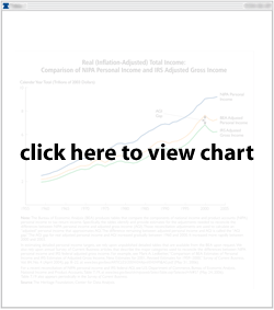
The difference remaining between adjusted personal income and AGI is called the "AGI gap." The total AGI gap for real adjusted personal income and inflation-adjusted AGI increased gradually between 1960 and 2000 (see Figure 6). It increased more rapidly between 2000 and 2003. However, the BEA's estimate of adjusted personal income captures most of the turning points in AGI. And differences between adjusted personal income and AGI are within ± 1.7 percent of the 12.3 percent mean difference for about two-thirds of the 45-year period shown in Figure 6.
The total AGI gap has been relatively constant in large part because the AGI gap for wage and salary income, has been historically stable. The size of the total AGI gap is influenced by wage and salary income because wages and salaries account for the largest share of both personal income and AGI. In 2003, wages and salaries were over 53 percent of NIPA personal income before subtracting employee-paid social insurance contributions. They were almost 74 percent of gross tax return income in 2003 and over 86 percent of the components of NIPA personal income included in AGI.
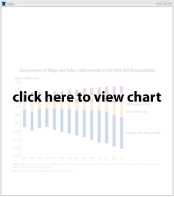
The definitional differences between NIPA wage and salary income and wages and salaries included in gross tax return income are numerous (see Figure 7). The NIPA definition includes wages and salaries that are not taxable, such as (some or tax-exempt) payments to military personnel, employee contributions to retirement programs (401K accounts, 403B accounts, TSP plans, etc.), and imputed estimates for non-cash income. It also includes earnings for individuals who do not file tax returns. However, it excludes income from disability pension plans and other sources included in taxable wages.
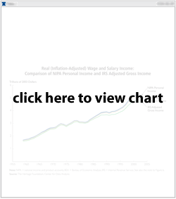
A comparison of the wage and salary components of adjusted personal income and IRS-reported AGI shows trends that are similar to those found in a comparison of total income (see Figure 8). For most of the period between 1960 and 2003, adjusted personal income moved in lock step with AGI wage and salary income, with a real mean overstatement of about 3.3 percent. As with total income, the AGI gap for wages and salaries in recent years has grown, in this case since 1996. By 2003, the adjusted personal income measure of wages and salaries overestimated its AGI equivalent by almost 7.5 percent, more than double the historical average. Nevertheless, we can derive a reasonably close relationship between NIPA and AGI wage and salary income by developing separate estimates for the reconciliation adjustments and the remaining AGI gap.[80]
In addition to being the largest component of NIPA personal income and AGI, wages and salaries constitute the greatest source of year-to-year variation in the NIPA-based portion of gross tax return income. For example, between 1990 and 2003, inflation-adjusted wages and salaries accounted for over 60 percent of the sum of annual absolute value changes in the income components of AGI that are also included in NIPA personal income.
Interest income is the second largest source of variation in the NIPA-based portion of AGI. Taxable interest accounted for around 15 percent of the absolute value inflation-adjusted annual change between 1990 and 2003. Unlike wages and salaries, the trend in interest income as measured in NIPA personal income is substantially different from the trend in interest income as measured in AGI. A large part of that difference may be attributed to the inclusion of imputed income in the NIPA -- but not the AGI -- measure of interest income. Imputed income comprised over 60 percent of NIPA personal interest in 2003.[81]
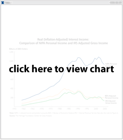
Even after subtracting imputed income and making other adjustments, some significant differences remain between the adjusted personal income measure of interest income and the AGI measure (see Figure 9). In general, the components of adjusted personal income, including interest income, are usually larger than the components of AGI. However, adjusted personal interest fell below the IRS measure in 1997 and 2000.
Dividend income is the third largest source of annual variation in the NIPA-based income portion of AGI. Between 1990 and 2003, dividend income was responsible for over 6.5 percent of the absolute value inflation-adjusted annual change in the NIPA components of AGI. However, important differences exist between the NIPA and AGI definitions of dividend income. For example, some payments to the owners of small business corporations (S-Corporations) are included in personal dividend income but excluded from IRS dividends. Such definitional differences complicate estimation of the income targets needed to calibrate the microsimulation model.
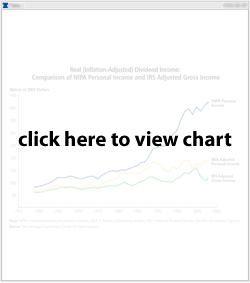
Even after the reconciliation adjustments are taken into account, both the level and movement of dividends in gross tax return income and NIPA personal income are noticeably different (see Figure 10). For example, between 2001 and 2002, AGI dividends fell by over $18 billion while the adjusted personal income measure of dividends showed an increase of over $20 billion, in inflation-adjusted terms.
A comparison of wage and salaries in adjusted personal income and AGI suggests a much closer relationship than evidenced for either interest income or dividend income. As a result, income estimates based on NIPA values are likely to be less accurate for the interest and dividend components of gross tax return income than they are for wages and salaries. Contributing to any potential inaccuracies, the Global Insight model does not include variables that can be used to estimate the reconciliation adjustments made by BEA when comparing NIPA personal income and IRS-reported AGI.
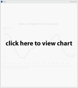
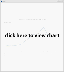
The effect of these limitations can be seen by comparing the actual amounts of gross tax return income and the estimated amounts obtained using a regression based on the historical relationships between the NIPA and tax measures. Most of the predicted amounts are close to their actual values. However, there are noticeable exceptions. For example, between 1993 and 1994, AGI interest income (including the non-taxable portion) was estimated to increase by roughly $20 billion to $191 billion (see Figure 11). Instead, actual AGI interest income fell by around $4 billion to $174 billion. Estimated dividend income in AGI and actual dividend income in AGI likewise diverged for several years between 1990 and 2003 (see Figure 12).
The paragraphs above discuss how we use NIPA data to estimate the amount of wage and salary income, dividend income, and interest income reported on tax returns. We use similar techniques to estimate other NIPA-based components of gross tax return income. Those components include proprietors' (farm and non-farm) gains and net losses, income from rents and royalties, and income from trusts and estates. We also estimate pass-through income from S-Corporations that is included in NIPA corporate profits.[82] Social Security income is introduced as a separate target because a portion of Social Security benefits are included in taxable income.
The sum of our forecasts of the components of NIPA-based income and non-NIPA-based income approximates the taxable income base that CBO uses to project federal receipts from the individual income tax. CBO does not provide its projections for most of the components of gross tax return income. As a result, there can be differences between income amounts we use and those projected by CBO. We do not have any information about the size of those differences, or whether they even exist, until we calculate federal revenues in the final step of the calibration process.
In the final step, we adjust a set of non-income variables used to calculate taxes in the model and introduce additional distributional targets. The non-income variables include itemized deductions and some statutory adjustments.[83] We compare CBO's projections of individual income tax collections with estimates of tax liability that are calculated by the microsimulation model and adjusted to reflect the timing of tax payments. Tax payments are divided into withholding, estimated payments, and final payments. The payments are aggregated to estimate fiscal year revenue collections. An additional adjustment is made to reflect payments for fees, penalties, and other collections. When there are material differences in the revenue projections, we modify our targets for the distribution of gross tax return income by size of income by marital filing status.
Adjustments may be needed because a large proportion of the total federal income tax is paid by a relatively small proportion of taxpayers at the top end of the income distribution. Slight changes in assumptions about the number of tax returns in the top classes can produce significant changes in total revenue projections. We do not know CBO's projections for the distribution of income or tax collections by detailed income class. We therefore adjust targets for both distributional variables in the final stage of calibrating the model so that estimates of total income tax collections from the microsimulation model approximate CBO's published projections.[84]
SECTION 4: IMPLICATIONS FOR TAX POLICY SIMULATIONS
An integrated calibration of the macroeconomic and microsimulation models provides a consistent basis for conventional tax policy analysis. The final CBO-like forecast replicates CBO's published projections (see Appendix A for additional details). It also includes projections of key components of NIPA personal income not typically published by CBO. The microsimulation model uses the final CBO-like forecast to generate current-law estimates of the federal income tax over a 10-year period. It includes detailed estimates by income class of gross tax return income on individual tax returns and non-taxable income as reported on the CPS. Those estimates of taxable and non-taxable income are consistent with components of NIPA personal income obtained from the final CBO-like forecast.
Calibrating the Global Insight model and the microsimulation tax model to a common starting point also produces a consistent basis for dynamic policy analysis. This is because an integrated calibration allows us to make direct comparisons between dynamically and conventionally estimated changes in federal income tax revenues. It also assures us that dynamic revenue estimates from the Global Insight model are broadly consistent with the microsimulation model's conventional estimates of revenue and distributional effects.
Our tax policy simulations broadly proceed in three separate steps once we have calibrated the Global Insight model and the microsimulation model to CBO's baseline projections.
First, we use the microsimulation model to obtain a conventional estimate of the revenue effects of a proposed change in tax policy. That proposed tax policy can involve a change in current-law federal income tax rates or provisions or a change in the federal personal income tax base. The microsimulation model is used to make a conventional estimate of the implied change in federal income tax revenues. It also produces estimates of marginal tax rates on three types of income -- ordinary income, long-term capital gains realizations, and dividend income -- under the proposed policy.
Second, we use the Global Insight model to estimate the dynamic revenue effects of the same policy change. We use conventionally estimated changes in federal tax revenues and marginal tax rates under current law and the proposed policy as inputs in a simulation with the Global Insight model. That simulation produces an alternative to the CBO-like baseline forecast. The alternative (non-baseline) forecast includes the dynamic effects of the proposed policy on GDP, prices, interest rates, employment, and personal and corporate incomes, among other variables. Revenue feedbacks can be calculated as the difference between the dynamically estimated change in federal income tax revenues from the Global Insight model and the conventionally estimated change in the same from the microsimulation model.
Third, we update the microsimulation model to reflect the dynamic effects of the proposed tax policy on personal and business incomes. We update personal and business incomes in the microsimulation model using similar procedures developed for baseline calibration. Thus, NIPA components of personal and business income along with price-level variables and some NIPA budget variables from the alternative forecast are used to estimate target values for gross tax return income on individual income tax returns and non-taxable income reported on the CPS. We use those targets to set personal and business incomes in the microsimulation model so that they are consistent with the Global Insight model's alternative forecast for the components of NIPA personal income.
We compare dynamically and conventionally estimated changes in federal tax revenues when evaluating results from the Global Insight model and the microsimulation model.[85] We consider the tax-policy simulation complete if differences between the Global Insight model's dynamically estimated changes and the microsimulation model's conventionally estimated changes in federal tax revenues can be accounted for by initial differences in the federal personal income tax bases in the two models.
In practice, we regularly calibrate both the Global Insight model and the microsimulation model to CBO's baseline projections. We also regularly use the calibrated macroeconomic and microsimulation models to analyze a variety of tax proposals. In some instances, tax data in the microsimulation model provide a "stand-alone" conventional revenue estimate. In other instances, the conventional revenue estimate is input into the Global Insight model to generate a "first-round" dynamic estimate of the economic and budgetary effects of the tax proposal. For a handful of major tax proposals, we have used the "first-round" dynamic estimate to re-age the matched file to reflect the new alternative forecast from the Global Insight model. When we have done so, we have iterated between the Global Insight model and the microsimulation model until the two models have produced similar revenue results.[86]
-- Tracy L. Foertsch, Ph.D., is a Senior Policy Analyst and Ralph A. Rector, Ph.D., is a Senior Research Fellow and Project Manager in the Center for Data Analysis at The Heritage Foundation. The useful comments of Mark A. Ledbetter (Bureau of Economic Analysis), Christopher Williams (Congressional Budget Office), Mark Lasky (Congressional Budget Office), and Rosemary Marcuss (Deputy Director of the Bureau of Economic Analysis) are gratefully acknowledged. The authors thank Kevin Kellert and Ben Keefer for their research assistance.
APPENDIX A: IMPLICATIONS OF CBO'S BASELINE PROJECTIONS FOR GDP AND PERSONAL INCOME
We use the final CBO-like forecast to infer values for key measures of macroeconomic activity and incomes. We focus here on two related issues -- the extent to which the January 2006 final CBO-like forecast reproduces key economic and budgetary projections published by CBO and the implications of those projections for the components of GDP and NIPA taxable personal income.
CBO publishes its projections for only a handful of the economic and budgetary variables comprising its current-law baseline. However for those projections CBO does publish, we ensure that the final CBO-like forecast replicates as closely as possible published values for every year in the 10-year budget period.
Table 2 gives calendar-year (and where appropriate fiscal-year) averages for a selection of variables included in the final CBO-like forecast. CBO publishes either levels or growth rate projections for a number of these, including nominal GDP (billions of dollars), real GDP (percent change from a year ago), the GDP deflator (percent change from a year ago), the CPI for all urban consumers (percent change from a year ago), the Employment Cost Index (ECI) for wages and salaries (percent change from a year ago), the 3-month Treasury bill rate (annualized percent), the 10-year Treasury note rate (annualized percent), the unemployment rate (percent of the civilian labor force), corporate book profits (billions of dollars), wage and salary income (billions of dollars), NIPA net federal government saving (billions of dollars), and unified federal surpluses (billions of dollars).
The final CBO-like forecast generally reproduces CBO's published economic and budgetary projections exactly. Exceptions include nominal GDP, NIPA net federal government saving, and unified federal surpluses.[87] Even then, however, the discrepancies between forecast values from the final CBO-like forecast and CBO's published projections are small. For nominal GDP, they average well under $1 billion between 2007 and 2016 and never exceed 0.02 percent of GDP (in absolute value) in any one year. For NIPA net federal government saving and unified federal surpluses, discrepancies average around $17.7 million between 2007 and 2016 and never exceed roughly $0.9 billion (in absolute value) in any one year.[88] They are almost entirely attributable to comparably small discrepancies between projections from the final CBO-like forecast and CBO's projections of NIPA federal receipts from personal and corporate income taxes.
Table 2 also gives forecasts from the final CBO-like forecast for several key macroeconomic and income variables excluded from CBO's published projections. Those forecasts include year-over-year percent changes in real personal consumption, residential and non-residential fixed investment, exports, imports, and government spending (federal as well as state and local purchases and gross investment). They also include nominal levels values for several components of NIPA taxable personal income used in the calibration of the microsimulation model -- namely, personal dividend income, personal interest income, personal rental income, proprietors' income (farm and non-farm).
We focus first on the largest component of GDP, personal consumption. The final CBO-like forecast puts growth in real consumer spending at 3.5 percent in both 2006 and 2007 (see Table 2). CBO forecasts the same growth rates in real consumer spending over the first two years of the 10-year budget period.[89] The final CBO-like forecast also incorporates a marked slowdown in the growth of real consumer spending between 2010 and 2011 (see Figure 13). That slowdown in real consumer spending is intended to be broadly consistent with the drop in personal disposable income implied by CBO's published projections of NIPA taxable personal income and NIPA federal receipts from personal income taxes (see Figure 1B and Table 2). It contrasts sharply with the GI control forecast's higher rates of growth in real consumer spending.
The final CBO-like forecast also implies a sharp drop in personal saving and the personal saving rate in the medium term (see Figure 14). Both the slowdown in the growth of real consumer spending and the decline in the personal saving rate are intended to reflect CBO's current-law assumption that tax relief provisions originally enacted under EGTRRA and JGTRRA expire in 2010. The GI control forecast assumes at least a partial extension of the expiring provisions of EGTRRA and JGTRRA. As a result, the personal saving rate in the GI control forecast is substantially higher than the projected personal saving rate implied by the final CBO-like forecast.
Projections for the remaining components of GDP do not so explicitly reflect current-law assumptions in the medium term. However, in most cases, we do attempt to ensure that they are broadly consistent with any additional details CBO makes available about its short-term forecast.[90] For example, non-residential fixed investment consists of business spending on equipment, software, and structures. The economic outlook chapter of The Budget and Economic Outlook indicates that in the short term CBO expects an "acceleration in the growth of structures relative to that of equipment and software."[91]
The final CBO-like forecast for business fixed investment seems broadly consistent with CBO's short-term outlook (see Figure 15). In it, the year-over-year percent change in real business spending on non-residential structures increases from just under 1.9 percent in 2005 to just over 10.0 percent in 2006. Over the same period, forecast growth in real business spending on equipment and software accelerates by far less. The economic outlook chapter also indicates that real business fixed investment expanded by around 9 percent in 2004 and 2005 and that "CBO forecasts similar growth for 2006 and 2007."[92] The final CBO-like forecast puts average growth in real business fixed investment at nearly 9.5 percent over the next two years.
Unfortunately, the final CBO-like forecast does not seem consistent with what we know about CBO's short-term forecast for state and local government purchases of goods and services. The economic outlook chapter indicates that CBO expects state and local government "spending to rise by roughly 2 percent in 2006 and 2007."[93] The final CBO-like forecast puts growth in real state and local purchases above 2 percent in both fiscal year 2006 and fiscal year 2007.
The final CBO-like forecast includes particularly strong growth in both real state and local gross investment and real state and local outlays for personnel.[94] Growth in either one could potentially be dampened during calibration, thus reducing overall growth in state and local purchases of goods and services. However, doing so would change projections of spending by all levels of government in the final CBO-like forecast.[95] It would also require adjusting other components of GDP -- possibly net exports -- so that in aggregate projected values of GDP remained consistent with CBO's published projections.
The final CBO-like forecast already seems roughly in line with what we know about CBO's short-term expectations for government spending and net exports. For example, CBO expects that "if current laws and policies do not change, such spending [real purchases for current consumption and investment by all levels of government] will grow by another 2 percent in 2006."[96] However, it expects that federal defense spending will to slow in 2007, "reducing the growth of the total purchases by the government sector."[97] The final CBO-like forecast puts growth in real purchases by government at all levels at a little over 2 percent in fiscal year 2006 and a little under 2 percent in fiscal year 2007. It puts the year-over-year percent change in real federal defense spending at -2.5 percent in fiscal year 2007.
Moreover, the final CBO-like forecast projects a trade deficit that is roughly stable. The nominal trade deficit measured as a simple difference between NIPA exports and NIPA imports levels off between 6.0 percent and 6.1 percent of GDP in 2006. It begins to decline gradually as a share of GDP in 2007. The economic outlook chapter indicates that CBO similarly expects that "the trade and current-account deficits will level off this year and then decline as a share of GDP over the medium term."[98]
We turn next to the components of taxable personal income (see Table 3A). Consistent with CBO's published projections, the ratio of wage and salary income to NIPA taxable personal income in the final CBO-like forecast is nearly constant over the 10-year budget period, never varying more than some 0.2 percentage point from a 10-year average of roughly 69 percent. However, income shares for the remaining components of NIPA taxable personal income drift slightly. For example, the ratio of personal dividend income and NIPA taxable personal income slips almost 1.4 percentage points over the 10-year budget period, declining to roughly 5.4 percent of NIPA taxable personal income by 2016. That decline in the personal dividend income share is largely offset by concurrent increases in personal interest income and personal rental income as a share of NIPA taxable personal income. It is most pronounced not after 2008 but in the second half of the 10-year budget period.
These changes in the composition of NIPA taxable personal income partly reflect trends in the GI control forecast -- but only partly (see Table 3B). Some components of NIPA taxable personal income in the final CBO-like forecast are set primarily using information from the GI control forecast. Thus, in both the control forecast and the final CBO-like forecast, personal interest income and personal rental income increase as a share of NIPA taxable personal.
However, the GI control forecast includes a roughly 4 percentage point drop in the ratio of wage and salary income to NIPA taxable personal income over the 10-year budget period. It also includes a slight upturn in the ratio of personal dividend income to NIPA taxable personal income. That increase in the personal dividend income share in large part mirrors trends in corporate profits in the GI control forecast. In contrast with CBO's baseline projections, corporate profits as a share of GDP rebound after 2011 in the GI control forecast. Consistent with the structure of the GI model, dividend income as a share of NIPA taxable personal income similarly rebounds.
Figure 1a.Figure 1b.
Figure 2.
Figure 3.
Figure 4.
Figure 5.
Figure 6.
Figure 7.
Figure 8.
Figure 9.
Figure 10.
Figure 11.
Figure 12.
Figure 13.
Figure 14.
Figure 15.
Table 1.
Table 2.
Table 3.
