Executive Summary

Over the past half-century, the American union movement has moved into government. Despite highly publicized efforts to curtail collective bargaining powers of government unions in Ohio and Wisconsin, almost all changes to government collective bargaining statutes over the past 20 years have increased, not decreased, the powers enjoyed by government unions.

This Special Report seeks to determine the extent to which unionization has increased the cost of state and local governments using three different econometric methods: (1) synthetic control, (2) regression analysis, and (3) Bayesian analysis. It includes a thorough review of statewide collective bargaining statutes across all 50 states and compares changes in these laws with changes in spending over the past six decades.

Using synthetic-control case studies, we find that collective bargaining significantly increased the cost of government for New York and New Jersey taxpayers, but had statistically insignificant effects in Ohio and South Dakota.

Expanding our analysis to use panel data for the entire country from 1957 to 2011, we find that mandatory collective bargaining increases government compensation, with little offsetting reduction in overall government employment. Instead, total state and local government spending increases by approximately $600 per person, per year. This represents a $2,300 greater annual tax burden on the average family of four.

Bayesian analysis shows an even larger effect, with mandatory collective bargaining increasing the cost of government operations by more than $750 per person, per year. This represents a $3,000 greater annual tax burden on the average family of four.

Across the United States, government unions increased spending by state and local governments by almost $127 billion in 2014, according to our regression results, and by $164 billion, according to our Bayesian results. These cost increases are concentrated in the states that grant the most aggressive powers to union leaders.

Introduction

The American labor movement was once concentrated in factories, mills, and other sites of private commerce. Few government unions existed until the 1950s. Today, half of American union members are government employees, not skilled tradesmen or factory workers.[1]

This shift partly reflects a decades-long decline in union participation among private-sector workers. It also reflects the fact that union participation rates for government employees increased sharply throughout the 1970s, and have remained stable at between 35 percent and 40 percent since the early 1980s.[2] The shift in union membership from the private sector toward government has important implications for public policy.

Government unions fundamentally differ from private-sector unions. They face little risk of losing customers if they demand too much, because the government compels taxpayers to purchase their services. Unlike private unions, government unions can help to select their own bosses. Politicians often reward government unions for their electoral assistance with higher compensation and higher staffing levels, even when politicians know these will strain public finances.

 

We begin with a review of the economic research on how government unions affect public finances and proceed to examine empirically how state and local government spending over the past five decades correlates with changes in government union powers. These powers are coded according to a hierarchy developed in the National Bureau of Economic Research (NBER) Collective Bargaining Law Data Set.

Our analysis reveals a direct relationship between government unions’ powers and the cost of state and local government operations. We estimate that states that extend mandatory collective bargaining powers to all state and local government employees spend $600 to $750 more per capita than states that do not. This raises the average cost of government by approximately $2,300 to $3,000 for a family of four.

We estimate that state and local governments would have spent $127 billion to $164 billion less in 2014 if none had enacted collective bargaining statutes for state and local government employees. In Appendix B, we provide information on the collective bargaining powers that government unions enjoy in each state, along with a brief legislative history of how they gained those powers.

How Government Unions Influence Public Policy

Government unions differ in many ways from their private-sector counterparts. Union organizing is easier in government because the government faces little competition.[3] This makes it easier for unions to charge taxpayers monopoly prices and deliver higher compensation to their members.[4] Government unions are also unique in that they can use political influence to select their own bosses.

Electoral Influence. Government unions have a massive influence in American political campaigns. They donate heavily to politicians that they support, their operatives volunteer on behalf of those campaigns, and their leaders encourage their members to vote as a bloc in favor of union-endorsed candidates.

These factors make a large difference. The Center for Responsive Politics reports that the second-largest donor to political campaigns nationwide since 1989 is the American Federation of State, County, and Municipal Employees. The fourth-largest donor is the National Education Association. The Service Employees International Union is the 10th-largest donor. These figures do not reflect additional, outside spending that unions also use to influence elections.[5]

Politician-Employers. Politicians have taken careful note of government unions’ ability to influence elections. Many politicians actively seek union political support. Some politicians will give government unions generous contracts in exchange for their help in getting elected. As labor economists Jeffrey Zax of Queens College and Casey Ichniowski of Columbia University observe, “The political objectives of government officials and of public employees may often be in concert rather than in conflict.”[6]

Harvard professor Richard Freeman suggests that this alignment of interests between government unions and their politician-employers is a major reason for the rapid growth of unions in government.[7] Instead of resisting union demands, politician-employers have a keen interest in encouraging unionization among government employees because the union political machines can help them to secure re-election.[ 8]

Fiscal Illusion. When government unions take such overt actions to control election outcomes, they expect compensation for their “political services.” However, as labor economists William Hunter and Carol Rankin explain, “the public has little interest in paying for political services…and thus politicians must make this compensation in a way that would not arouse public scrutiny.”[9]

Politicians can reward unions in non-obvious ways by using multiple unique pay categories to supplement base wages or salaries. For example, many government unions negotiate premium pay, allowances, and other categories, such as “longevity pay,” that are generally foreign to the private sector. In addition, politicians reward unions with generous deferred-compensation packages, including pension and health benefits for retirees. The complex accounting behind these perks makes it difficult for the public to easily understand the full cost of what politicians and unions have negotiated. Additionally, in the case of deferred-compensation packages, the full cost usually does not encumber public finances until long after the politicians leave office.

George Mason University research fellow Eileen Norcross refers to these practices as “fiscal illusion” because unions and politicians use them to intentionally obscure the public’s understanding of government compensation.[10]

Lobbying. Government unions differ from their private-sector counterparts not only in their ability to select their own bosses, but also in the fact that they can increase the demand for their services through effective lobbying. Most economists agree that private-sector unions face a trade-off between higher wages and fewer jobs. Through lobbying and marketing campaigns, government unions can increase the demand for government services, thereby securing both higher wages and greater employment simultaneously.

Bradley University economist Kevin O’Brien has examined this practice in detail and confirmed that the lobbying efforts of government unions increase government employment. O’Brien examined data for municipal police and fire departments nationwide and found that departments with collective bargaining agreements paid 13 percent to 14 percent higher wages, but that lower employment offset the higher wages, leaving total spending unchanged—consistent with standard economic theory. When these unions engaged in lobbying, however, staffing levels increased, resulting in greater department spending.[11] O’Brien concludes:

It appears that if a public employee union wants to increase its employment and wage bill, having a collective bargaining agreement is not sufficient—public employee unions must also be politically active.… Thus, political activities by unions can be viewed simply as a means to escape the wage-employment trade-off imposed on bargaining outcomes by the demand for labor.[12]

How Do Government Unions Affect Government Spending?

If government unions can increase government compensation while increasing government employment, unionizing government should increase government spending. Scholars have spent decades trying to answer just how much unions increase government spending.

In doing so it has become clear that government unions’ leverage is closely tied to the strength of their legal powers of compulsion. In other words, unions increase compensation and staffing levels in government the most when the law requires government employers to negotiate with them and to submit to a compulsory dispute-resolution process.

The Legal Environment. For this reason, researchers quickly realized that they would need to evaluate the degree to which state collective bargaining laws empower government unions. This allowed scholars to then estimate how changes in the law affected key outcomes, such as union density, government compensation and employment levels, and total government expenditures.

Robert Valletta, an economics professor at University of California, Irvine, and Harvard economist Richard Freeman, director of Labor Studies for the NBER in 1988, constructed the NBER Collective Bargaining Law Data Set.[13] The dataset extends back to 1955 so that researchers can measure changes in the law over time. Economists have updated it several times. In addition, the dataset maintains a coding unique to each of five different employee groups: (1) state workers, (2) local schoolteachers, (3) local police, (4) local firefighters, and (5) other local employees.

Freeman and Valletta analyzed Current Population Survey (CPS) data from the Census Bureau using this collective bargaining data. They found that “state public sector laws are a prime determinant of the likelihood that municipal workers are covered by collective bargaining.” Strong collective bargaining laws were also associated with higher government wages and staffing levels. They concluded: “We find that employment and wages in otherwise identical departments are higher in those with collective bargaining contracts, supporting the notion that public sector unions raise demand for labor as well as increase wages along given demand curves.”[14]

Princeton economist Henry Farber subsequently updated the NBER dataset through 2004.[15] Farber made some simplifying changes, using an ordinal 1–8 scale:

1. Collective bargaining prohibited.
2. No legal provision for collective bargaining.
3. Collective bargaining permitted, but not required.
4. Public employers are required to “meet and confer” with union leaders.
5. Public employers have a compulsory duty to bargain collectively, express or implied.
6. Collective bargaining is compulsory and mediation is required.
7. Collective bargaining is compulsory and strikes are protected.
8. Collective bargaining is compulsory and arbitration is required.

Farber concedes that it is unclear whether a protected right to strike or a required arbitration process grants greater leverage to unions, although it is reasonable to characterize arbitration as the higher form of compulsion because it is the only mechanism that guarantees a union contract. Farber found that his simplified scale strongly correlated with the key variables of interest, with coefficients similar to those found in other studies. For instance, his analysis concludes: “Compared to there being no legal provision, [government employee] earnings are 5 to 15 percent higher where the employer has a legal duty to bargain.”[16]

The current analysis extends this NBER dataset forward to 2011 in order to examine the financial impact of collective bargaining laws over a longer period and in more recent times, and to compare changes in state law with changes in state and local government spending.

Compensation and Employment. Among the most notable contributions in the research on unions and government pay, Freeman reviewed all previous studies and found that the financial impact of government unions grew over time. Later studies noticed larger differences between the compensation levels of governments that engaged in collective bargaining and the levels of those that did not. Freeman also confirmed that a preponderance of studies found that unionization causes governments to hire more workers, with “the most comprehensive study”—a comparison of 400 cities over a decade by Zax[17]—showing that unionization increases public employment by about 10 percent.

Freeman concludes: “Still, on the basis of the existing estimates of the effect of unions on employment, wages and budgets…, it is likely that public sector unions raise both taxes and public services above what they would be in the absence of unions.”[18]

Other researchers come to similar conclusions. Bahman Bahrami, John D. Bitzan, and Jay A. Leitch compare the wages of union and non-union government workers between 1998 and 2004 using CPS data. They controlled for differences in educational attainment, years on the job, and other personal characteristics. Using a sample size of nearly 130,000 government employees, they find that unionized local-government workers enjoy a wage premium between 14.6 percent and 17.4 percent, while unionized state-government workers enjoy a wage premium between 10.7 percent and 12.5 percent. Interestingly, they also found that about 40 percent to 50 percent of the differences in wages between government and private-sector workers can be attributed to differences in their qualifications or characteristics, while 50 percent to 60 percent of the difference is due to fundamental differences in the way government workers are compensated.[19]

In a subsequent study published in 2010, Bitzan and Bahrami used this dataset to examine the union effect on government wages by occupation, and compared these pay rates directly with private-sector equivalents. They generally find that public-sector pay for management positions is comparable with pay for management positions in the private sector, but that other, non-management occupations have far higher pay levels than their private-sector counterparts.[20] Table 1 reproduces some of the occupational premiums for unionized government that they identified.

 

Total Government Spending. While the union impact on wages and benefits is interesting, the question remains: Do government unions increase overall government spending?

Some analysis suggests they may not. Zax and Ichniowski examined how collective bargaining affected total government spending for 463 cities across five years and found ambiguous results. They found that collective bargaining increased spending on various functional areas between 5 percent and 16 percent, but that local governments at least partly offset these higher costs by cutting employment in non-union departments. For example, municipalities offset higher costs in unionized fire departments by hiring fewer non-union sanitation workers.[21]

We re-examine this question, using the updated NBER dataset on collective bargaining laws and total government expenditures, both by function area and in the aggregate. We examine annual state and local government spending from 1957 to 2011, a period spanning the introduction of all statewide collective bargaining laws. Appendix A explains how we compiled these data.

Several recent studies have examined the relationship between union density and total government spending. For instance, Michael L. Marlow and William Orzechowski found that every percentage-point increase in union coverage rates during the mid-1980s increased per-capita state and local government spending between $6.97 and $10.01.[22] All else equal, the results indicate that increasing government union density from 10 percent to 40 percent would increase government spending by $200 to $300 per capita.

In a later study, Marlow examined the relationship between union coverage rates and per capita spending by state and local governments during the mid-2000s, using similar control variables. He found that every percentage-point increase in union coverage rates led to an increase in state and local government spending of $38.39 per capita.[23] Accordingly, increasing government union density from 10 percent to 40 percent would imply a $1,150 increase in per capita state and local government spending.

Our results strengthen these findings and find similar results. We unambiguously find that government collective bargaining laws are a primary factor in determining government spending levels. We find that per capita government spending rises by $500 to $750 in states that mandate collective bargaining in the governments’ workforce.

Synthetic-Control Case Studies

We begin our analysis with four case studies that examine how requiring mandatory collective bargaining affected per capita state and local government spending in Ohio, New York, South Dakota, and New Jersey. Appendix A explains in detail why we selected these states, along with additional results from the synthetic-control analysis that we employ.

Synthetic-control case studies allow researchers to compare a treated state to a mathematically optimal group of control states in which public policy did not change. Comparing the actual states’ experience with its “synthetic” counterpart shows the effect of the public policy change, in this case requiring state and local governments to collectively bargain.

New Jersey. Chart 2 shows the results of this analysis for New Jersey. Our synthetic New Jersey closely matches per capita spending in New Jersey before the state required collective bargaining. After passage of compulsory collective bargaining laws, the two diverge markedly. A decade later, New Jersey’s state and local governments spent $846 more per person (in 2011 dollars) than in the counterfactual New Jersey without government unions.

 

Of course, these results could occur simply due to random chance. To determine the statistical significance of a synthetic control case study, economists run the “experiment” again for every state that did not undergo a policy change. They compared how much the treated state varied from its counterfactual to how much the other states did.

Chart 2 also shows the results of this “placebo test.” The thick line represents the difference between the synthetic New Jersey and the actual New Jersey, and the vertical line represents the year of treatment. The thin lines show the difference for those states that did not mandate collective bargaining in 1968 or thereafter.

The largest treatment effect occurs with the treated New Jersey. This effect is unusually large, larger than all of the placebo tests. It roughly equates to significance at the 5 percent level using conventional tests of statistical significance. Notably, over time, the distance between the synthetic New Jersey and the actual New Jersey widens. Government unions have significantly raised costs for New Jersey taxpayers.

New York. They appear to have done the same in New York. By 1978, New York state and local governments spent approximately $1,000 more per capita (in 2009 dollars) than did synthetic New York. This result is also statistically significant. Chart 3 shows that in the decade after New York passed its law, none of the placebo states experience an effect size as large as New York’s.

 

Ohio. Chart 4 shows the results for Ohio. We do not find as good a synthetic match for Ohio as for New Jersey or New York. However, after the treatment period, the difference between the synthetic Ohio and the actual Ohio grows. By 1995, government spending per capita is over $400 higher in Ohio than in its synthetic counterpart. However, these results are not statistically significant. Two other states had larger effect sizes in the placebo tests.[24] Consequently, the Ohio results are not statistically significant at conventional levels.

 

 

South Dakota. Like Ohio, our synthetic control estimates for South Dakota also found that granting unions compulsory bargaining powers slightly increased government spending. Chart 5 shows those results. By 1981, government spending had risen just under $100 more per capita in actual South Dakota than in synthetic South Dakota. Like for Ohio, this finding was not statistically significant. Most of the placebo states exhibited equally large effect sizes despite not having passed comprehensive collective bargaining reforms in this period.

 

Regression Analysis

The cases studies presented here provide suggestive, but not conclusive, evidence that collective bargaining increases government spending. Drawing firmer conclusions requires more comprehensive analysis. In this section, we report the results of regression analysis on panel data of state and local government spending for all 50 states between 1957 and 2011. In the following section, we analyze these data using regression analysis.

We find certain notable trends across all employee classes:

First, laws giving government unions greater powers of compulsion correlate with higher wages for the employees to which they apply.

Second, collective bargaining laws have a small impact on employment levels, which lacks statistical significance in several cases. These findings are consistent with previous literature that indicates unions can escape the wage-employment trade-off by using political activism to increase overall demand for public employment.

 

Third, stronger collective bargaining powers are associated with higher total government spending, not just higher pay. Reduced spending within non-union departments does not appear to entirely offset the higher labor costs in unionized departments. Giving unions powers of compulsion raises costs for taxpayers.

We present the results for the impact of collective bargaining laws on each of these variables below for each of the five major employee classes. We present results for each relationship using four different statistical approaches, including ordinary least squares (OLS) regression, under both random effects and fixed effects, and Driscoll-Kraay standard errors regression, with and without fixed effects. Our preferred specification is column 4, which accounts for state fixed effects and controls for possible geographic correlations between states. All dollar figures are inflation-adjusted to 2009 dollars using the gross domestic product deflator. Appendix A provides a detailed discussion of the statistical methodology, choice of variables, and other technical concerns.

State Workers. As seen in the first row of Table 2, a movement of one interval along the NBER scale for state workers correlates with an increase in state employee monthly pay per full-time equivalent (FTE) position in the range of approximately $25 in three of the four models, and those increases are highly statistically significant. The Driscoll–Kraay model without fixed effects finds only a marginally significant increase in state employee pay. This variable only measures wages and salaries and excludes benefits such as health care or retirement contributions.

The second row examines the impact of a one-interval movement along the NBER scale on state employment per capita, as measured by the number of FTE positions filled by state governments. While all results are significant at the 1 percent level, the models all show that changes in state collective bargaining laws have a very modest impact on state government employment.

These results imply that an upward movement along the NBER scale increases the overall taxpayer wage bill for state employees: average pay increases without any drop in employment. This does not necessarily mean that overall state spending will increase. The state may offset higher labor costs by reducing spending elsewhere.

The results in the third row of Table 2 show that such reductions do not fully offset the higher labor costs. Stronger legal powers for state employee unions increase overall state spending. Per capita state spending rises by $89 to $105 for every one-increment movement up the NBER scale. On average, a state that moves from prohibiting collective bargaining to requiring it with arbitration for state employees—increasing seven increments along the NBER scale—sees per capita costs of state government increase between $625 and $735.

The fourth row shows that total spending by state and local governments combined rises by an amount roughly equal to the spending increase at the state-government level alone when state employee unions receive more aggressive powers of compulsion.

These spending increases may reflect more than compensation increases for state employees. States that require collective bargaining for state employees often require collective bargaining for local government employees as well. A substantial portion of local government spending in many states is financed by transfers from the state government. Higher state spending may also reflect concurrent spending increases caused by unionization of local governments. We later specify a model accounting for all collective bargaining laws simultaneously.

As we discuss in Appendix A, government spending may not change linearly as states move up the NBER scale. We suspected that certain key points along the scale would have a larger fiscal impact than others. While there is clear precedent within the academic literature for using the linear NBER scale and our own analysis confirms its usefulness, we also examined the differences between states with mandatory bargaining (those scoring between 5 and 8 along the NBER scale) and states without mandatory bargaining (those scoring between 1 and 4).

 

Those results, presented in Table 3 for state workers, confirm a significant divergence between states with compulsory bargaining and those without it. States with compulsory bargaining for state government employees pay between $105 and $144 more monthly per FTE position, while total employment increases slightly.[25] Total state spending also increases between $420 and $500 per capita. All of these results are highly statistically significant.

K–12 Employees. We performed a similar series of analyses regarding the impact of collective bargaining laws for K–12 educational employees. This group includes teachers, administrators, and support staff. We found results similar to those for state employees.

As seen in the first row of Table 4, every one-increment movement up the NBER scale increases cash pay per FTE position in K–12 education between $13 and $21. These values are statistically significant at the 1 percent level using three of four regression techniques, but only marginally significant using Driscoll–Kraay standard errors with a fixed-effects specification. These pay increases have little effect on overall employment in the K–12 sector. Per capita FTE employment barely changes.

 

The third row of Table 4 shows some evidence that greater legal powers for education unions have little statistically significant effect on K–12 education spending. The OLS regressions find that each movement up the NBER scale increases spending by approximately $5 per capita. However, these regressions do not account for geographic correlations between states. The Driscoll–Kraay regressions, which do account for this potential correlation, show no statistically significant effects on K–12 education spending.

We found it curious that the coefficient on total K–12 spending was so much smaller than the relationship for collective bargaining powers for state employees. One possible explanation is that teacher unions may deploy their lobbying powers to increase government spending generally and, thus, create externalities that benefit other government unions while not internalizing all of the benefits of their actions.

The fourth row of Table 4 suggests that this occurs. At a minimum, it indicates that states do not offset higher K–12 compensation with reduced spending in other functional areas. In fact, every one-increment movement up the NBER scale for teachers is associated with a rise of $41 to $47 in per capita spending by state and local governments.

Focusing solely on the impact of mandatory bargaining laws tells a similar story. As seen in Table 5, compulsory bargaining for education employees is associated with a small rise in per capita spending on K–12 of approximately $37 under the OLS specification. The first Driscoll–Kraay model returns statistically insignificant coefficients. Our preferred specification, the Driscoll–Kraay model with fixed effects, shows a marginally significant positive effect of collective bargaining on K–12 education spending. The second row further shows that compulsory bargaining for education employees is associated with a rise in total spending by state and local governments of $175 to $243. These results are statistically significant, although the results in column 3 are only significant at the 10 percent level.

 

Firefighters. The first and second rows of Table 6 show that every one-increment movement up the NBER scale for firefighters is associated with an increase in monthly pay per FTE fire position of $36 to $61 with minimal negative impact on employment.

This rise in pay translates into minimal increases in fire protection spending per capita, as seen in the third row of the table. As with teacher unions, the fourth row shows little support for the notion that reduced spending on non-union functions offsets higher spending on unionized fire departments. Every one-increment movement up the NBER scale for firefighters correlates with an overall increase in local government spending of $48 to $71. In this case, we focus on local government spending because the bulk of firefighting spending occurs at that level, whereas spending on K–12 occurs at both the state and local government levels.

 

Compulsory bargaining laws for firefighters show a larger effect. States with compulsory bargaining laws for firefighters tend to have higher spending on fire protection of $5 to $6 per capita, as seen in the first row of Table 7. These increases are all statistically significant. These states are also associated with a rise in total spending by local governments of $207 to $295 per capita, as the second row shows. This could reflect spillover effects from firefighter union lobbying on the general demand for government services. It could also reflect states requiring collective bargaining with firefighters at the same time that they require it for other local government employees.

 

Police. Every one-increment movement up the NBER scale for police is associated with an increase in monthly pay per FTE police position of $50 to $69 with a small impact on total employment, as seen in the first two rows of Table 8.

This greater spending on police wages produces a statistically significant increase in total police spending of $2 to $3 per capita, as the third row of Table 8 shows. As with teachers and firefighters, total spending by local governments—where the bulk of police spending occurs—rises even faster than spending on police alone. The bottom row of Table 8 shows that spending by local governments rises by $32 to $42 with every one-increment movement up the NBER scale for police unions.

This consistent finding that spending increases considerably more overall than in particular departments that unionize undercuts the notion that spending reductions in non-union departments entirely offset the spending increases that unions cause. Indeed, for each employee class, greater powers for unions correlate with a larger rise in total government spending than in spending on the affected function alone.

 

Table 9 focuses solely on the difference between states with and without compulsory bargaining statutes for police unions. They show compulsory bargaining results in a rise in police spending of $12 to $18 per capita and increases total spending by local governments by $176 to $182 per capita.

 

Other Local Government Employees. We analyze local-government employee groups that do not fall into one of the prior employee classes together in Table 10. These include transit workers, sanitation workers, social workers, and other civil servants. The first and second rows show that each step up the NBER scale for these unions correlates with a $15 to $24 increase in monthly pay per FTE position. These pay increases come with a minimal impact on employment.

 

This rise in wages has no statistically significant effect on spending on these functional areas in three of the four model specifications, but total local government spending does rise appreciably.

Looking solely at the difference between states with and without compulsory bargaining statutes for these employees, Table 11 shows that localities with compulsory bargaining statutes for other local employees tend to spend $194 to $248 more per capita.

 

Average of Collective Bargaining Laws. These regressions show that expanded collective bargaining powers have a greater effect on overall spending than on the unit directly affected. This holds true for every class of employees except state government workers. This could indicate that the political activities of government unions increase the overall demand for government.

However, it could also reflect the fact that states tend to expand collective bargaining powers for multiple groups of employees at the same time. For example, Michigan required local governments to bargain with all employee groups—police, fire, educational, and “other” employees—in one bill in 1965. Regressions analyzing expanded collective bargaining powers for police employees on total spending conflate the effect of the police unions with the effect of other unions who gained these powers at the same time.

To estimate aggregate impact of changes in collective bargaining laws for all employee groups on state spending, we construct an interaction term that averages the values for each occupational group for each state in each year. Appendix A explains the construction of this interaction term in greater detail.

The results, in Table 12, show that when all occupational groups simultaneously experience a one-increment increase in the strength of bargaining laws, monthly pay per FTE government position increases by $23 to $35, depending on the statistical method. This increase is statistically significant in all of the models examined. The second row shows that this change has a limited impact on overall employment levels.

 

The third and fourth rows of Table 12 show that this simultaneous one-increment increase across all five employee classes results in increased per capita spending by local governments of $38 to $53 and by state governments of approximately $100. These spending increases are statistically significant in all specifications.

However, we cannot simply sum these impacts to determine the total impact on spending by state and local governments because of intergovernmental transfers. State-level appropriations fund much local government spending. The fifth row of Table 12 shows the results of a simultaneous one-increment increase across all five employee groups on total state and local spending net of this intergovernmental spending. A simultaneous one-increment increase in union power translates into a statistically significant increase in total spending by state and local governments of $117 to $146 per capita.

We also examined the difference between states with and without compulsory bargaining statutes for all five employee classes.[26] Table 13 shows that monthly pay per FTE position in states with compulsory bargaining laws is $76 to $134 greater than in states without these laws, with minimal impact on employment. The coefficients for monthly pay are significant at the 1 percent level using three of four statistical techniques. However, the Driscoll–Kraay model with fixed-effects specification is only marginally significant.[27] Per capita state and local government employment changes minimally.

Table 13 shows that compulsory bargaining laws for all employee classes are associated with an increase in local spending of $169 to $200 per capita, and an increase in state spending of $532 to $561 per capita.

 

 

Net of intergovernmental spending, state and local governments combined tend to spend $573 to $720 more per capita where collective bargaining is compulsory across all five employee groups. This increase is highly statistically significant. It translates into an additional tax and spending burden of $2,300 to $2,900 on an average family of four.

These findings present concrete evidence that state collective bargaining laws granting strong powers of compulsion to government unions have added significantly to the cost of state and local government operations over the past five decades.

Bayesian Analysis

This regression analysis provides strong evidence that collective bargaining powers increase the cost of government services. However, regression analysis has shortcomings. The statistical theory underlying this analysis assumes that the parameters in statistical models are fixed quantities. These methods rely heavily on large sample approximations by assuming asymptotic normality, and that the observed data are a single realization of infinitely many samples. Bayesian methods, on the other hand, assume that the parameters are random variables to which a priori assumptions are assigned via probability distributions.

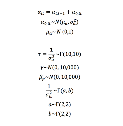
To assess the robustness of our regression results, we also estimated five Bayesian statistical models. These Bayesian models analyzed the impact of these control variables—including the NBER collective bargaining scale—on the levels of per capita state and local government expenditures. Some of these models, described in detail in Appendix A, made different assumptions about whether these variables had different effects in different states. In addition, Models IV and V included a time-varying dynamic component in their intercept terms to model the concept that there may be a certain degree of time dependence occurring between years. Table 14 shows our coefficient estimates in terms of posterior means. Appendix A presents more detailed results, including posterior standard deviations and Bayesian credible interval estimates.

 

These results indicate that a movement of one interval up the average NBER scale for all state and local employees correlates with a $105 to $228 increase in per capita government expenditures. We computed pseudo-Bayes factors, also discussed in Appendix A, to compare our model’s explanatory power. We found that Model V has the best predictive ability, while Model IV best fits the data. Model IV estimates that each increment a state advances along the NBER collective bargaining scale increases per capita state and local government spending by approximately $150. Model V estimates that each increment a state moves up that scale increases spending by approximately $225.

These Bayesian models find that collective bargaining has a larger effect on government spending than the regression analysis found. The preferred estimates in Table 14 are larger than the comparable regression estimates in the fifth row of Table 12. Our preferred estimate—model IV—implies that mandatory collective bargaining increases state spending by over $750 per capita. For example, one may consider a state that moves from an average of 2 on the NBER scale (no legal provision for collective bargaining in government) to an average of 7 (mandatory collective bargaining with strikes permitted). The estimates in column IV imply that state and its local governments would see their total annual spending increase by over $750 per capita. That means collective bargaining causes taxes to rise by more than $3,000 for the average family of four.

Total Effect on State Spending. Across all states, the average NBER strength of collective bargaining laws in 2011 was 5.13.[28] Based on the spending trends over the past five decades, if state and local governments had never granted such powers of compulsion to union leaders in the public sector (maintaining an NBER value of 2), the regression estimates indicate those governments nationwide would have spent $127 billion less in 2014 alone, with savings concentrated among the states with the most aggressive bargaining laws for government workers. The Bayesian model suggests that taxpayers would have saved $164 billion that year.[29]

Conclusion

Many, but not all, American states have given unions considerable power over government employees and government operations. Government unions can frequently force workers to accept their representation, require state and local governments to bargain with them, and prevent non-union workers from working for terms outside the union contract. These powers enable unions to increase compensation for government employees.

Private-sector unions face a trade-off between higher wages and fewer jobs for their members. Studies find that government unions avoid this trade-off through political activism. Their lobbying and political activities raise the demand for government services overall, enabling them to raise government pay without reducing government employment.

However, it is not clear that this raises total costs to taxpayers. Some previous research has suggested that governments offset higher costs in unionized departments with spending cuts elsewhere, leaving overall government spending little changed.

This Special Report comprehensively analyzes changes in state and local government spending between 1957 and 2011. It shows that government unions unambiguously raise total costs for taxpayers. Spending cuts elsewhere do not fully offset the costs associated with unionizing government. States that give unions collective bargaining powers increase total spending by an average of $600 to $750 per capita. Government unions cost the average family of four between $2,300 and $3,000 per year.

Nationwide, states’ decisions to give government unions collective bargaining powers have inflated spending by state and local governments, and imposed a significant fiscal burden on taxpayers. Our results indicate that somewhere between $127 billion and $164 billion in 2014 spending by these governments is attributable to public-sector collective bargaining rules—with these additional costs concentrated among the states that award the most aggressive powers to unions.

—Geoffrey Lawrence was Director of Research at the Nevada Policy Research Institute until January 2015. He left NPRI in January 2015 and is now the Assistant State Controller of Nevada. James Sherk is Research Fellow in Labor Economics in the Center for Data Analysis, of the Institute for Economic Freedom and Opportunity, at The Heritage Foundation. Kevin D. Dayaratna, PhD, is Senior Statistician and Research Programmer in the Center for Data Analysis, of the Institute for Economic Freedom and Opportunity, at The Heritage Foundation. Cameron Belt was previously a Research Assistant at the Nevada Policy Research Institute. He is now Senior Economist at RCG Economics, LLC.

Appendix A: Statistical Methodology

This study uses panel data for all independent and dependent variables for all 50 states between 1957 and 2011.[30]

We tested whether the legal environment for public-sector collective bargaining arrangements had an effect on the level of per capita government expenditures, payrolls, and full-time-equivalent (FTE) workers.

Choice of Independent Variable

While previous studies have focused on union density as a possible determinant of government spending, we focused on the strength of collective bargaining laws. By examining only union membership, previous analysts implied that a union’s size alone determines how much influence it has over public policy. However, government unions exert strong influence on public-policy decisions because they enjoy powers not enjoyed by other citizens, not simply through the size of their membership. For this reason we believe that the legal framework is a more suitable indicator of union power.

Furthermore, these two variables are highly correlated. Union density tends to be highest where unions enjoy the strongest powers of compulsion. We found that changes in the legal environment account for roughly 80 percent of the variation in government union density. In practice, the choice of either variable has little impact on our results. The strong correlation between legal powers and union density prevents us from including both variables simultaneously without creating problems with multicollinearity.

Choice of Additional Control Variables

We assembled panel data for each state and year from 1957 through 2011. We included controls for factors other than union power that could affect government financial decisions. The difficulty in obtaining annual state-level data back to 1957 limited our choice of control variables. We considered, but could not find enough data for, controls for the unemployment rate, poverty rates, and racial and linguistic demographics. Each of these variables could influence government spending by increasing the demand for government services. We instead used the number of FTE workers employed in state and local welfare divisions as a proxy for variations in the demand for government services.

We also included controls for a two-period lag of the log of state population, the log of personal disposable income, right-to-work status, the political party in power in the governor’s office, and a second-order polynomial time trend.

Both population and per capita personal income can significantly affect government expenditures.[31] Controlling for personal income per capita accounts for individual state economic conditions, such as state costs of living and economic growth. The two-period lagged growth rate of state population helps to control for growth in the demand for infrastructure spending and other public services and for a growing tax base. We use lagged data because government budgets and expenditures do not vary immediately with changes in population. Generally, the increased demands of population growth take time to change state and local government budgets. Population changes in the current year do not usually influence the current year’s budget. Moreover, we normalized the dependent variables into per capita figures. Including the current period’s population as a control variable could lead to complications from regressing on an identity. We chose a two-year lag because some states do not set budgets on an annual basis and because statistical tests showed that longer lags did little to explain variation in the dependent variables.

Researchers have, unsurprisingly, found that the political preferences of the electorate affect government spending decisions. To account for this, we include a dummy variable that has the value of 1 when a Democrat holds the governor’s office. We also include dummy variable for whether a state has a right-to-work law. This variable may have a direct economic effect, but it also serves as a proxy for public attitudes toward unions.

We considered and chose to exclude other control variables that may appear relevant. For example, previous studies have controlled for regional factors (such as whether the state is in the South), population density, and the overall state and local tax burden.

Regional factors remain constant through time and are captured by our fixed-effects estimator. Some previous studies analyzed Southern states separately because of a perceived “anti-union” cultural value. This might make sense if union density was our independent variable. However, the legal environment for government collective bargaining varies greatly throughout the country, including among Southern states. As such, we saw no reason to isolate Southern states and treat them differently.

Previous studies have analyzed whether population density affects the size of government, positing that denser areas have a greater demand for public services and infrastructure spending. However, while population density may be an appropriate measure when comparing municipal expenditures, we believe it only confuses the results when applied at the state level. For example, Western states have lower population density than the Eastern states, but several Western states have high government spending.

We did not expressly adjust for cost-of-living differences because our fixed effects estimator accounts for such state-specific effects. The variable for personal income per capita also partly accounts for it; wage differences between states largely reflect differences in living costs.

Finally, using the tax burden as a control variable makes little sense when government spending is the dependent variable: 49 states (all states except Vermont) have a balanced budget requirement that restricts state-level spending to the amount of available revenue.

Model

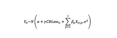
Having selected the appropriate variables, our model takes the form:

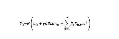
Yikt = α+ γ (CBLawikt)+ β(Xit) + εikt

where Y is the level of per capita spending, FTEs, and payrolls in state i at time t in sector k (Total, State, Local, Police, Other, and Fire). Furthermore, CBLawikt is the collective bargaining regime, Xit is the vector of control variables, εikt is the error term, and α is a fixed-effects dummy variable.

We normalized all relevant government expenditures, FTE employment levels, and total payrolls by adjusting them into per capita terms.

We present our results using ordinary least squares (OLS) in columns 1 and 2 of Tables 2–13. Panel data has the potential to introduce potential complications that could bias our estimated coefficients and attenuate standard errors, particularly heteroskedasticity, serial correlation, and cross-sectional dependence. We corrected for these problems using Driscoll–Kraay standard errors. Monte Carlo tests have shown that Driscoll–Kraay standard errors best correct these problems in panel datasets with large numbers of panels and large time series.[32] We present the Driscoll–Kraay results in columns 3 and 4 of Tables 2–13.

The model also needed to account for possible state-specific factors that could affect the variables of interest. We tested for whether estimators of state-specific fixed effects or random effects were appropriate, and found the fixed-effects estimator was the appropriate specification. The results in columns 2 and 4 of the tables display these fixed-effects estimators under OLS and Driscoll–Kraay standard errors, respectively. For the sake of completeness, we present the random-effects estimator under OLS standard errors in column 1.

Using a fixed-effects model introduces other potential complications. It eliminates differences across states and restricts identifying variation to differences within states over time. This may eliminate valuable identifying information. To address these concerns, we also ran the models without fixed effects using pooled data and with the Driscoll–Kraay robust standard errors (not a random-effects specification). We present these results in column 3 of Tables 2–13. The general similarity of the results in column 3 and column 4 provides evidence that our model is correctly identified. While we present multiple estimates, our preferred estimates are the Driscoll–Kraay standard errors with fixed effects in column 4.

We tested for unit roots in our data using the Levin–Lin–Chu test recommended for use in moderate-sized datasets.[33] These tests indicated stationarity in three of the dependent variables we examined: (1) local government FTE police employment per capita; (2) total government FTE police employment per capita; and (3) real K–12 spending per capita. The test rejected the null hypothesis of a unit root for all other dependent variables.

For the sake of presentation, we display only the regression coefficient on the collective bargaining variables in Tables 2–13. The full regression results, obtained using STATA 13, are available upon request.

Data Sources

We obtained historical data on union bargaining powers by state and year from the NBER collective bargaining scale. We updated these data through 2011. We also compiled data on the date of the enactment of state right-to-work laws and the years in which states had Democratic governors. We obtained state per capita personal income data from the Bureau of Economic Analysis. We obtained data on annual state populations from the Census Bureau.

For our dependent variables, we used different functional job classifications of real government spending, FTE employees, and payroll, all normalized by state population. We defined average earnings as the average monthly earnings for employees within the selected category. These earnings figures do not include benefits, such as pensions or health care. In all, our variables include total, state, local, and specific department (police, fire, teachers, and other) spending, payrolls, and employment.

We obtained these data from the Census Bureau’s Annual Survey of State and Local Government Finance. This annual survey began in 1977, and we merged it with the Census of Governments survey starting in 1957. For non-survey years from 1957 to 1977, the Census Bureau provides estimates of annual values. We interpolated the remaining missing observations.

We adjusted the dependent and independent variables for inflation (2009 dollars) using the gross domestic product (GDP) deflator.

Additional Considerations

One potential limitation on our model is its implicit assumption that each incremental movement along the NBER scale affects government expenditure by an equal magnitude.

We attempted a functional form using a separate dummy variable for each of the eight NBER levels of collective bargaining. Our coefficients on these dummy variables were generally statistically insignificant. This is likely due to the lack of enough variability within and across panels for each of these dummy variables to capture and explain variations within our dependent variables. For example, 70 percent to 95 percent of the separate state collective bargaining individual-level dummies are 0. However an F-test of joint significance was performed for each model. The F-test returned a p-value of 0.00 for all models. So while the dummy variables for the NBER bargaining scale are not individually significant, they are jointly significant, and we can reject the hypothesis that they have no effect on the outcome variables. Because of this result, we followed the precedent within the literature that uses this 1–8 scale as an independent variable.[34]

Nonetheless, we felt compelled to further clarify the analysis identifying the points along the NBER scale that have the greatest impact on government expenditure. Our intuition was that the greatest impact came from granting compulsory collective bargaining. We created and tested a new dummy variable equal to 1 when the collective bargaining variable was greater than or equal to 5—indicating mandatory collective bargaining—and equal to 0 when the value was 4 or less.

Using this variable in our model produced statistically significant results. In our main results, we present these results along with the results using the NBER scale. For the estimates looking at total state and local government spending across all employee classes, we created a variable equal to 1 if all five employee groups had compulsory collective bargaining powers, and 0 if they did not. In this way, we differentiated states giving the strongest powers to government unions from those that did not. While this may seem a restrictive definition, approximately one-third of all state-year observations fit this classification. In results not shown, we created a variable summing the total number of compulsory bargaining laws across all five employee classes. Using this variable, we found similar results to those presented in the paper.

Robustness Tests

We tested the robustness of our principal finding—that greater powers for government unions increase total government spending—to alternative model specifications.

Semi-Log Model. The first two rows of Appendix Table A-1 replicate the models used in the final row of Tables 12 and 13, respectively. They differ only by examining the log of per capita total state and local government expenditures as the dependent variable instead of the level of those expenditures.

Both the NBER collective bargaining scale and the dummy variable indicating whether a state mandates collective bargaining for all employee groups show a statistically significant correlation with higher government spending. The first row of Appendix Table A-1 shows that under the semi-log specification, a one-unit increase in the NBER collective bargaining scale increases total state and local government spending between 0.7 percent and 2.1 percent. This implies that total government spending would increase between 5 percent and 15 percent if a state moved up all seven units in the NBER scale.[35] Our preferred Driscoll–Kraay fixed-effect estimate implies a 5 percent increase in total government spending.

The second row of Appendix Table A-1 shows that states requiring collective bargaining for all employee groups have 3 percent to 8 percent higher total spending than states that do not.[36] The preferred Driscoll–Kraay fixed-effects specification implies 3 percent greater government spending in these states, and the result is statistically significant at the 1 percent level.

 

Dropping Control Variables. Appendix Tables A-2 and A-3 replicate the Driscoll–Kraay with fixed-effects regression on total government spending from Tables 12 and 13, respectively. The last column shows the complete regression results from the models in Tables 12 and 13. The remaining columns show the results of iteratively dropping each control variable in the analysis. Both the analyses using the NBER collective bargaining scale and mandatory collective bargaining for all employee groups are robust to the exclusion of most control variables. However, the NBER-scale analysis is not robust to excluding the time trend from the analysis.

Census Division Specific Time Trends. Given the necessity of controlling for time trends, we believe it important to include a time trend. However, we also explored the robustness of our results to alternative specifications of the time trend. In the third and fourth rows of Appendix Table A-1, we replicate the total government spending results from Tables 12 and 13, using a second-order polynomial time trend for each census division, rather than a nationwide time trend. This somewhat reduces the magnitude of the results, but all coefficients remain statistically significant at conventional levels.[37]

 

 

Case Studies Using Synthetic-Control Approximation. The ideal study would have a set of control states and exactly identical treatment states before the treatment period and administer the treatment at exactly the same time. This research design would provide a truly unbiased treatment effect. As is frequently the case in economics, this has not happened in the real world. We instead created a synthetic experiment using the synthetic-control method.

The synthetic-control method is primarily used in comparative case studies. It uses a data-driven procedure to create a best-matched counterfactual from a group of control states that accurately mimics the treated state in the time period prior to treatment. The method compares the observed, actual dependent variable data (for instance, per capita spending) in the post-treatment period with the created, unobserved synthetic-control observations from the best-matched group of control states in an attempt to provide a relevant counterfactual to understand what overall effect the treatment (such as a collective bargaining policy change) had on the treated state.

For the purposes of this analysis, the best possible treatment groups are states that mandated compulsory collective bargaining for all five employee classes simultaneously. In total, 10 states passed compulsory laws for all five employee groups at the same time: New York (1967), Washington (1968), New Jersey (1968), Oregon (1969), Hawaii (1970), South Dakota (1970), Minnesota (1971), Montana (1973), Florida (1974), and Ohio (1984).

We compared these states with a control group of states that either never had any compulsory laws or have never had more than two compulsory collective bargaining laws at a time. (We attempted to use a control group made up of states never exposed to compulsory collective bargaining laws, but were unable to make relevant synthetic-control groups for any of our 10 treatment states.) Appendix Table A-4 provides the complete list of control states and the number of employee categories with compulsory bargaining.

 

Among the treated 10 states, we were able to create four synthetic-control matches that accurately reflected the traits of the treated units in the pre-treatment period. While we would have preferred to examine more states, the data-driven procedure of the synthetic-control method statistically determined whether a state was a good candidate for analysis.

We could not create a statistically representative match in the other six states with the available pool of control states. When tested, the six states produced root mean square prediction errors (RMSPEs) ranging from two- to seven-times higher than our best fitting model, New Jersey.

State legislatures typically pass legislation in the middle of the year, and the legislation usually takes effect several months later. For example, the New York legislature passed the Taylor Law requiring collective bargaining in the state and local government in April 1967. The law took effect in September 1967. For the purposes of our analysis, we considered the treatment to begin in the first full year after the collective bargaining law passed.[40] This avoids conflating inaction before the law takes effect with the law having no effect. Following Abadie, Diamond, and Hainmueller’s pioneering work on synthetic control case studies, we constructed synthetic control matches for a decade following the initial passage of the collective bargaining law.[39] They explain that a decade is “a reasonable limit on the span of plausible prediction” under the synthetic-control method.[40]

For each state we constructed our synthetic-control match on the level of per capita state and local government spending one, five, and 10 years before the treatment took effect, the log of real GDP per capita, the log of real personal income per capita, the log of state population, and the average strength of all collective bargaining laws in place.

Charts 2 through 5 present the results of these synthetic control analyses. In each state, government spending grew faster in the actual state that required collective bargaining than in the synthetic state that did not.

To test for statistical significance, we conducted placebo tests. This involved replicating the synthetic experiment on states that did not change their collective bargaining laws. We compared the difference between the synthetic and actual states from these placebo runs with the difference for the states that changed their collective bargaining laws. Charts 2 through 5 also display the placebo tests for each of the states under analysis.

Both New Jersey and New York showed statistically significant increases in government spending. The difference between the actual and synthetic real per capita government spending grew at a faster rate in those states than in any of the placebo tests. Real per capita state and local government spending grew faster in Ohio and South Dakota than in their synthetic states, but these differences were not statistically significant.

Appendix Table A-5 shows the weights on each state used in the synthetic control matches. Appendix Table A-6 shows how closely the synthetic states match the actual states in the pre-treatment period for the matched characteristics.

 

Bayesian Analysis

We tested the robustness of our regression results using Bayesian analysis. Standard frequentist approaches assume that the parameters in statistical models are fixed quantities. These methods rely heavily on large sample approximations by assuming asymptotic normality and that the data observed are a single realization of infinitely many samples. On the other hand, Bayesian methods assume that each parameter’s true value is a random variable to which a priori assumptions are assigned via a probability distribution.[41] Based on both the sample data as well as the prior information, a posterior distribution regarding each parameter can be estimated conditionally on observed data.

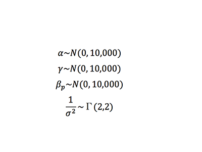
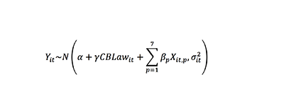
We estimated five Bayesian statistical models (Models I–V) to understand the impact of a variety of factors—in particular, the presence of right-to-work laws, the political party in power, time, income, population, government welfare spending, and the presence of collective bargaining laws—on the level of per capita government expenditures. Models I–V differed in assumptions regarding heterogeneity of intercepts as well as error terms. In addition, Model IV and Model V included a time-varying dynamic component in their intercept terms to model the concept that a certain degree of time dependence may occur between years. We present below detailed results from this Bayesian analysis, including posterior standard deviations and Bayesian credible interval estimates.

Model 1

 

With prior specification:

 

Model 2

 

With prior specification:

 

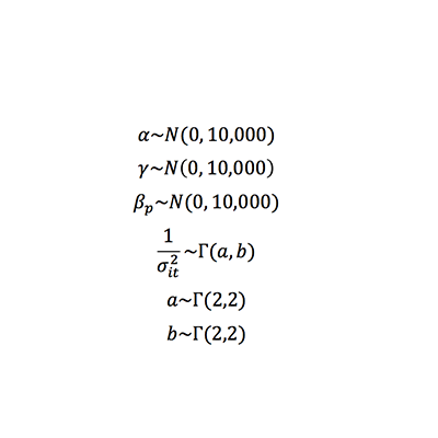
Model 3

 

With prior specification:

 

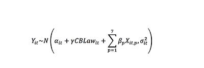
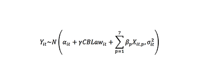
In these models, for state i and time t, Xit,1 is a binary variable indicating the presence of right-to-work laws, Xit,2 is a binary variable indicating whether the governor is a Democrat, Xit,3 represents time, Xit,4 represents time squared, Xit,5 represents the natural log of per capita personal income, Xit,6 represents the two period lagged state population, Xit,7 represents all government welfare spending for full-time employees, CBLawit represents the state’s score on the NBER collective bargaining scale, and Yit is per capita government spending.

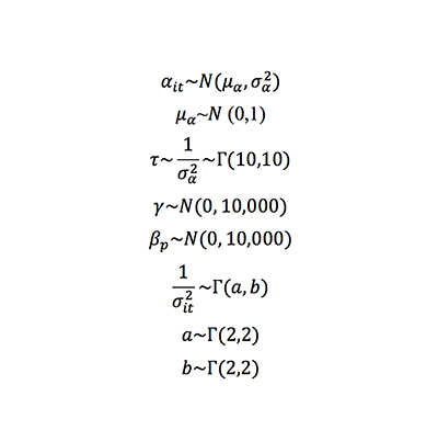
Model 4

 

With prior specification:

 

Model 5

 

With prior specification:

 

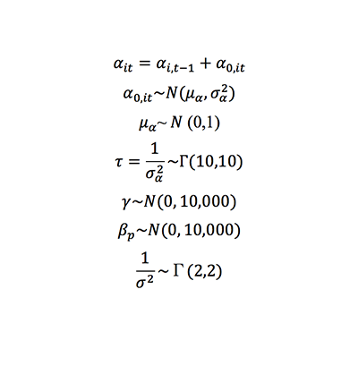
Our models differ in intercept and variance. Model IV and V introduce a dynamic component by allowing a time-varying intercept term. Posterior distributions of the parameters in the models were estimated via the Markov Chain Monte Carlo (MCMC) simulation, using over 20,000 MCMC iterations with an additional 5,000 for burn-in. We ensured convergence to a stationary distribution by monitoring the time series of the iterations. Posterior means, standard deviations, and credible intervals are reported. We tested the robustness of our results for a variety of prior distributions beyond those specified above and found results similar to those presented here.

 

It is useful to assess the comparative predictive ability of our five models. Bayes factors are generally used for this purpose. The pseudo Bayes factor (PsBF) is based on a model’s cross-validation predictive density. As standard Bayes factors are often not computationally feasible to compute, the PsBF is considered a useful surrogate.[42] We computed PsBFs for Models II–V to compare them to Model I. We also checked within sample error by computing Mean Absolute Error (MAE) of the predictive posterior distribution. Both are presented in Appendix Table A-12:

 

These results suggest that Model V has greater predictive ability than its counterparts, while Model IV has the best fit in terms of within sample error. Model IV indicates that each increment a state advances along the NBER collective bargaining scale increases state and local government expenditures by approximately $150 per capita. Model V indicates that each step along the NBER scale is associated with spending approximately $225 higher per capita.

Appendix B: State-by-State Analysis

Appendix B provides a brief historical background on collective bargaining laws in each of the 50 states and applies the findings from our statistical analysis to draw conclusions about the impact that changes to the law might be expected to produce in each state.

This appendix focuses on statewide laws on government unions. We recognize that local governments in some states engage in collective bargaining with their employees despite no legal requirement to do so.

Judicial opinion has been divided as to whether local governments can engage in collective bargaining if the state legislature has not granted them the authority to do so. For instance, Virginia’s Supreme Court declared that local governments could not engage in collective bargaining without state authority, whereas Florida’s Supreme Court concluded otherwise. In either case, a state statute expressly authorizing collective bargaining clearly grants more leverage to government unions than the absence of one, and this distinction has been discussed at length in the academic literature.

We also provide an overview of the current labor law environment for each class of government employees, along with a ranking system that provides context for the unique provisions in each state.

Appendix B also creates a new metric for comparing the labor law environment (LLE) for government employees across the 50 states based on what the statistical analysis developed in this paper reveals to be some of the most significant variations in state collective bargaining statutes. An LLE score, ranging from 0 to 1, is computed for each state. Scores near 0 mean government unions have few powers of compulsion, while scores near 1 indicate that they have the greatest available powers of compulsion over government employees.

These scores are calculated in rough proportion to what the authors observe to be the most significant variables in state labor laws based on the results of empirical analysis developed for this paper. Specifically, a state’s LLE score is composed of:

• NBER score for the collective bargaining regime (50 percent);
• Right to work versus forced unionization (20 percent);
• Dispute-resolution mechanism (10 percent);
• Legality of strikes (10 percent); and
• Proportion of government employees covered by a union contract (10 percent).

The LLE score allows meaningful comparisons across states using a single, ratio-scale variable. Accordingly, the authors have used this new metric to rank the states based on their LLE score. Every state falls within a range of 0.013 to 0.898. States lower on this scale award fewer compulsory powers to public-sector unions and, thus, earn a higher ranking.

Virginia ranks first due to its explicit prohibitions against any coercive powers for public-sector unions, right-to-work provisions, and low union-participation rates among government workers. At the other end of the spectrum are 19 states with LLE scores greater than 0.8, with Pennsylvania ranking last.

This appendix also analyzes the prospective fiscal impacts that would result from a change in collective bargaining regimes in each state. We provide a range of figures, using the coefficients from the final row of column 4 of Table 12 and the third row of column 4 of Appendix Table A-1 that estimate the correlation between average collective bargaining powers and total state and local government spending per capita. We multiplied these coefficients by the Census Bureau’s 2014 state population estimates, the change in average collective bargaining powers, and adjusted for inflation between 2009 and 2014 to arrive at our estimate of the change in total state and local government spending.

These spending changes do not exclusively reflect spending on compensation for government employees. Government unions campaign extensively for higher taxes and against spending cuts. Their members capture some, but not all, of the financial proceeds of this lobbying. For example, in 2012, government unions in California funded a ballot measure to increase state income and sales taxes. It passed, and the state and local governments spent more than they would have in 2013. Our estimates capture the overall effect of government unions on government spending, including spillovers that increase spending outside unionized departments.

Alabama

LLE Score = 0.180

RANK: 6

Background. In June 1957, Alabama prohibited government-sector collective bargaining for all employee groups. Lawmakers partially reversed course 10 years later, when they required public employers to meet with firefighter union representatives to discuss their proposals for contract terms. Beginning in 1996, a similar requirement was imposed on local school boards, which became obliged to “meet and confer” with teacher union representatives.

Analysis. For three of five employee groups, Alabama explicitly prohibits public employers from signing contracts with union leaders. This prohibition undergirds the state’s LLE score of 0.180, ranking sixth among the states for restricting government unions’ powers of compulsion.

However, if Alabama lawmakers had never reversed the prohibition against collective bargaining for teachers and firefighters, state and local spending for 2014 would likely have been between $349 million and $739 million less in 2014. On the other hand, if the powers of compulsion currently enjoyed by teachers and firefighters had been expanded to other employee groups, 2014 spending would likely have been about $524 million to $1.1 billion higher. If all employee groups had received the most aggressive powers of compulsion (an NBER score of 8), 2014 spending would likely have been $1.6 billion to $3.6 billion higher.

Alaska

LLE Score = 0.888

RANK: 49

Background. Alaska lawmakers enacted the state’s first collective bargaining statute in April 1959, giving state and local governments the option of bargaining collectively with union representatives. By June 1970, teacher union bosses successfully prodded lawmakers to grant them compulsory collective bargaining powers along with the explicit right to strike. In September 1972, those powers were extended to unions representing all employee groups. A subsequent change in 1993 removed the explicit power to strike from police and firefighting professionals and replaced it with a binding arbitration process.

Analysis. Lawmakers in Alaska have done little to restrict government unions’ powers of compulsion over public employers, having granted compulsory bargaining along with coercive resolution techniques to every class of union. Alaska’s labor environment for government workers is among the most coercive in the nation.

If collective bargaining had remained optional for Alaska’s public employers, state and local government spending in 2014 would have been about $239 million to $585 million lower. If no collective bargaining law had ever been implemented, 2014 spending would have been about $282 million to $599 million lower. By contrast, if all employee groups had gained access to a mandatory arbitration procedure, 2012 spending would have been between $26 million to $57 million greater.

A right-to-work law would have reduced government spending by around $234 million.

Arizona

LLE Score = 0.313

RANK: 12

Background. Teacher union leaders prompted Arizona lawmakers to pass the state’s first formal collective bargaining statutes in 1973, making it optional for local school districts to enact collective bargaining ordinances. Similar powers were extended to all other employee groups beginning in 1975. In December 2008, Governor Janet Napolitano (D) issued an executive order requiring state agencies to engage in a “meet-and-confer” process with unions for state workers. Governor Jan Brewer (R) rescinded the order four months later.

Analysis. Although many local jurisdictions in Arizona participate in collective bargaining or a meet-and-confer procedure, Arizona’s statewide legal regime imposes few obligations on public employers to negotiate with unions.

If lawmakers had gone the other direction and explicitly prohibited collective bargaining, 2014 spending would have been about $808 million to $1.7 billion lower.

On the other hand, if public employers had been required to engage in compulsory collective bargaining and mandatory arbitration with all unions, 2014 spending would have been $2.1 billion to $4.2 billion greater.

Arkansas

LLE Score = 0.264

RANK: 8

Background. Lawmakers in Arkansas enacted the state’s collective bargaining statute in September 1968, which formally gives local governments the option of engaging in collective bargaining or passing ordinances that require collective bargaining. Although lawmakers revised the statute slightly in 1983, the law has remained mostly unaltered.

Analysis. Arkansas ranks alongside Arizona, Louisiana, South Carolina, and West Virginia as states that give public employers the option of negotiating with unions for all employee classes.

If Arkansas had never granted public employers explicit authority for collective bargaining, state and local government spending in 2014 would likely have been about $178 million to $398 million lower. If lawmakers had gone the other direction and explicitly prohibited collective bargaining, 2014 spending have been about $357 million to $754 million lower.

On the other hand, if public employers were required to engage in compulsory collective bargaining and mandatory arbitration with all unions, 2014 spending would have been $890 million to $1.8 billion greater.

California

LLE Score = 0.813

RANK: 34

Background. California’s first collective bargaining statute was passed in September 1962, requiring state agencies, local school districts, and fire departments to “meet and confer” with union leaders. For police, collective bargaining remained optional. However, a subsequent change to the law in 1969 granted compulsory collective bargaining powers with mandatory mediation to all municipal unions. These new powers were extended to teacher unions in 1976 and to state workers beginning in 1992.

Analysis. Today, unions representing all employee groups enjoy compulsory collective bargaining powers, and public employers are required to submit to mediation to resolve disputes. This legal regime mirrors closely those found in Florida, New Hampshire, and South Dakota.

If these coercive powers had never been granted to unions in California, state and local government spending in 2012 would likely have been $9.3 billion to $19.7 billion lower. If lawmakers had gone the other direction and expressly prohibited government-sector collective bargaining, 2014 spending would have been $11.6 billion to $24.2 billion lower.

Colorado

LLE Score = 0.463

RANK: 20

Background. Colorado’s first statewide collective bargaining law did not become effective until 1977, and it gave school districts the option of bargaining with teacher unions. For local police, firefighters, and other municipal unions, Colorado has never enacted a formal collective bargaining law. In November 2007, Governor Bill Ritter (D) issued an executive order requiring state agencies to sign collective bargaining agreements with government unions and to submit to mandatory mediation. The order was prompted, in part, by the unions’ threat to picket the 2008 Democratic National Convention in Denver if they were not given such powers.

Analysis. The compulsory collective bargaining powers awarded to unions for state workers in 2007 drastically altered Colorado’s labor law environment. If this executive order were rescinded, Colorado’s LLE score would return to 0.388, and the state’s national ranking would improve to 16th.

If Colorado expressly prohibited government-sector collective bargaining, 2014 spending would have been between $644 million and $1.4 billion lower. On the other hand, if the powers that state-level unions currently enjoy had been granted to all municipal and teacher unions, 2014 spending would have increased by the same amount.

Connecticut

LLE Score = 0.862

RANK: 41

Background. Unions for teachers, police, firefighters, and other municipal workers acquired compulsory bargaining powers with mandatory arbitration when Connecticut lawmakers passed the state’s first collective bargaining law in June 1965. Legislation in October 1975 extended these powers to unions for state workers. Little has changed since then.

Analysis. Along with eight other states, Connecticut has granted compulsory bargaining powers combined with mandatory arbitration to unions for all five employee groups.

Based on our findings, an across-the-board reduction of these special powers for government unions could yield substantial savings. If lawmakers simply had removed coercive forms of dispute resolution, but retained compulsory bargaining, state and local spending in 2014 would have been about $648 million to $1.4 billion lower. If government-sector collective bargaining had been prohibited, 2014 spending would have been $1.5 billion to $3.2 billion lower.

Delaware

LLE Score = 0.840

RANK: 37

Background. Delaware’s first collective bargaining law, passed in September 1964, gave state agencies the option of negotiating with unions for state workers. Union powers were strengthened substantially the following year when unions for state, police, firefighter, and other municipal workers were granted compulsory bargaining powers combined with mandatory arbitration. In somewhat atypical fashion, teacher unions were the last to acquire these powers. Compulsory bargaining with required mediation was granted to teacher unions in 1969, but not until March 2008 did teacher unions receive the powers of mandatory arbitration.

Analysis. Along with eight other states, Delaware now has the highest possible composite score for the strength of unions’ legal powers of compulsion. Unions for all five employee groups enjoy compulsory bargaining combined with mandatory arbitration.

An across-the-board reduction of these special powers for government unions could yield substantial savings. If lawmakers had simply removed all coercive forms of dispute resolution, but retained compulsory bargaining, state and local spending in 2014 likely would have been about $169 million to $357 million lower. If all provisions for collective bargaining simply had been removed from state law, 2014 spending would have been $337 million to $713 million lower.

Florida

LLE Score = 0.580

RANK: 24

Background. Collective bargaining powers were first bestowed on government workers in Florida through a controversial Florida Supreme Court decision in 1968. The decision in Dade County Classroom Teachers Association v. Ryan followed a series of illegal work stoppages by government workers throughout the 1960s, including the nation’s first statewide teacher strike in 1968. Subsequent legislation in 1975 formalized these powers into law, granting unions for all employee groups compulsory bargaining powers along with required mediation.

Analysis. Florida is unique as the only Southern state to grant such aggressive powers of compulsion to unions representing all groups of government workers. The average LLE score for all other Southern states is 0.208, which underscores the regional uniqueness of Florida’s laws.

If Florida had simply made collective bargaining optional across all employee groups, 2014 spending would have been between $3.6 billion and $7.6 billion lower. A Virginia-style prohibition on collective bargaining for government workers would have yielded a 2014 savings of $6.0 billion to $12.7 billion. However, if Florida’s dispute-resolution mechanisms were changed from required mediation to binding arbitration, 2014 spending likely would have been $2.4 billion to $5.1 billion greater.

Georgia

LLE Score = 0.203

RANK: 7

Background. Georgia’s experience with government-sector collective bargaining has been sporadic. The state’s first law, passed in September 1966, formally gave school districts the option of bargaining with teacher unions. However, in 1970, lawmakers expressly prohibited bargaining with unions for state workers. The following year, lawmakers granted firefighter unions compulsory bargaining powers with mediation required. Then, in 1974, lawmakers changed course again, expressly prohibiting collective bargaining with teacher unions.

Analysis. Express prohibitions against collective bargaining with teacher and state employee unions conflict with the aggressive powers of compulsion granted to firefighter unions. If Georgia lawmakers had extended these express prohibitions to all government unions, state and local government spending in 2014 would have been between $849 million and $1.8 billion lower.

By contrast, if unions for all employee groups had received the same powers enjoyed by firefighter unions, 2014 spending would likely have been between $1.5 billion and $3.4 billion greater. If unions for all employee groups had obtained compulsory bargaining powers along with the power to compel public employers to submit to binding arbitration, 2014 spending would have been $3.4 billion to $7.2 billion greater.

Hawaii

LLE Score = 0.711

RANK: 30

Background. Hawaii passed its first statewide collective bargaining law in July 1970, which instantly awarded compulsory bargaining powers to all government unions, along with a mandatory arbitration procedure guaranteeing union contracts. In an interesting twist, Hawaii’s law simultaneously granted the explicit right to strike to unions for state workers, teachers, and municipal workers other than police and firefighters. Typically, states that provide a binding arbitration procedure to government unions do not also allow those unions to strike.

Analysis. Along with eight other states, Hawaii has granted unions for all five employee groups compulsory bargaining powers combined with mandatory arbitration. However, Hawaii is unique in granting government unions a protected right to strike alongside a binding arbitration procedure. Typically, arbitration is seen as a method of avoiding strikes by guaranteeing union contracts.

If lawmakers had imposed compulsory bargaining without the mandatory arbitration or striking provisions, state and local spending in 2014 would have been between $255 million and $541 million lower. If no collective bargaining law had ever been enacted, 2014 spending would have been between $511 million and $1.1 billion lower.

Idaho

LLE Score = 0.420

RANK: 17

Background. Idaho’s first collective bargaining laws took effect in 1960 and gave local governments the option of engaging in collective bargaining with police, firefighter, teacher, and other municipal unions. Changes to the law in 1970 and 1971 granted greater powers to firefighter and teacher unions. Both were granted compulsory bargaining powers and could force their employers to submit to a mediation or fact-finding procedure. In 1978, firefighters also gained the explicit right to strike. This is atypical, in that public safety workers are rarely awarded the explicit right to strike. No law has been enacted governing state employee unions.

Analysis. Aggressive powers of compulsion awarded to Idaho’s firefighter and teacher unions stand in contrast to those for other employee groups. If Idaho lawmakers had simply reverted to the 1960 law that allowed optional bargaining for these groups, state and local government spending in 2012 would have been between $117 million and $249 million lower. If lawmakers had expressly prohibited collective bargaining for all employee groups, 2014 spending likely would have been $314 million to $664 million lower.

On the other hand, if union powers for all other employee groups were expanded to match those for firefighters, 2014 spending likely would have been $373 million and $811 million greater.

Illinois

LLE Score = 0.883

RANK: 47

Background. Beginning in 1967, public employers in Illinois received explicit statutory authorization to engage in collective bargaining. Unions representing state workers led the charge in Illinois, gaining compulsory bargaining powers with mediation required in 1973. In 1984, unions for teachers and municipal workers other than police and firefighters gained this power as well, and all received explicit legal protections for strikes. Not until 1996 did police and firefighter unions gain compulsory bargaining powers with required mediation. Three years later, these powers were expanded to include mandatory arbitration.

Analysis. A highly publicized 2012 Chicago teacher strike, in which thousands of teachers shut down city streets with demonstrations, served as a nationwide reminder of what can happen when state law enshrines public workers’ abilities to strike or engage in other militant action.

If lawmakers had never granted these powers to unions, but unions still enjoyed the power of compulsory bargaining (an NBER score of 5), state and local spending in 2014 likely would have been about $1.8 billion to $3.9 billion lower. If no collective bargaining statute had ever been enacted in Illinois, 2014 spending would have been about $4.1 billion to $8.8 billion lower. With an express prohibition on bargaining, 2014 spending would have been $5.0 billion and $10.4 billion lower.

Indiana

LLE Score = 0.327

RANK: 13

Background. Indiana passed its first formal collective bargaining law in August 1969, giving explicit authority to state agencies and local governments to bargain with unions for all employee groups. Legislation in 1973 required school districts to bargain with teacher unions. When Mitch Daniels (R) became governor in 2005, he issued an executive order on his first day in office prohibiting state agencies from bargaining with state employee unions, and that prohibition remains in place. However, legislation enacted later that year required school districts to submit to mediation with teacher unions. In 2011, those powers were broadened to require binding arbitration.

Analysis. Indiana stands in sharp contrast to neighboring Illinois, Michigan, and Ohio. With teacher unions as a lone exception, Indiana has shown far greater restraint in granting legal powers of compulsion to government unions.

Indiana taxpayers could still realize substantial savings if lawmakers extended the prohibition on bargaining to all state employee unions across the board. If they had done so for 2014, spending likely would have been $870 million to $1.8 billion lower.

Iowa

LLE Score = 0.644

RANK: 29

Background. Iowa lawmakers crafted the state’s first collective bargaining statute in 1970, formally giving state and local governments the option of negotiating with government unions. In 1975, lawmakers eliminated the option and imposed compulsory bargaining and mandatory arbitration on local governments for all four classes of local government workers. The following year, the same requirements were imposed on state agencies. No major changes to the law have occurred since then.

Analysis. Along with those in eight other states, Iowa lawmakers have granted compulsory bargaining and mandatory arbitration powers to unions for all five employee groups.

Iowa’s long-standing provisions empowering government unions have been a central reason for the rapid growth in the per capita cost of state and local government. Between 1992 and 2012, that inflation-adjusted figure grew from $3,796 to $9,897. If lawmakers had granted compulsory bargaining powers to all unions, but refrained from imposing mandatory arbitration on public employers, 2014 spending by state and local governments likely would have been about $560 million to $1.2 billion lower. If the legislature prohibited government-sector collective bargaining, 2014 spending would have been $1.3 billion to $2.7 billion lower.

Kansas

LLE Score = 0.367

RANK: 16

Background. Teacher-union leaders secured strong powers of compulsion from Kansas lawmakers in July 1970, when the state’s first collective bargaining statute immediately awarded them compulsory bargaining powers as well as mandatory arbitration. Two years later, lawmakers passed the first formal laws for other employee groups, giving local governments the option to negotiate with union leaders while requiring a meet-and-confer process for state agencies. Interestingly, the 1972 law includes detailed language describing a binding arbitration process for local governments if they decide to bargain collectively, but city councils and county commissions can opt out of the whole process.

Analysis. If collective bargaining with teacher unions had remained optional for school districts as with other local governments, state and local government spending for 2014 would likely have been $209 million to $442 million lower. If collective bargaining were expressly prohibited, that figure would be between $558 million and $1.2 billion.

However, if the powers currently held by teacher unions had been granted to all unions, 2014 spending would likely be $662 million to $1.4 billion greater.

Kentucky

LLE Score = 0.597

RANK: 26

Background. Kentucky’s first collective bargaining law became effective in February 1965 and explicitly authorized school districts to bargain with teacher unions. The following year, lawmakers expressly prohibited collective bargaining within state agencies. In 1972, lawmakers granted police and firefighter unions compulsory bargaining powers. Additional changes in 1998 and 2004 required fire and police departments, respectively, to enter mandatory mediation. Governor Paul Patton (D) created the Employee Advisory Council by executive order in 2001, essentially establishing a meet-and-confer process for state workers, who came to be represented by the Teamsters. Upon becoming governor in 2003, Ernie Fletcher (R) rescinded the order, but Governor Steve Beshear (D) reissued it in early 2008 after winning the governorship with Teamster support.

Analysis. If Kentucky lawmakers had never given compulsory powers to police and firefighter unions, state and local government spending for 2014 would likely have been $317 million to $673 million lower. However, if the powers currently held by police and firefighter unions had been granted to all unions, 2014 spending likely would have been $477 million to $1.0 billion greater.

Louisiana

LLE Score = 0.313

RANK: 11

Background. Legislation in April 1972 explicitly authorized state agencies and local governments in Louisiana to collectively bargain with union leaders. The legislation followed a series of strikes by teacher unions in New Orleans throughout the late 1960s, including a 1969 strike in which union operatives formed an “anarchy committee” that made headlines by slashing tires and igniting explosives on school grounds in an effort to pressure school district officials into agreeing to union demands. No major legislative changes have occurred since 1972.

Analysis. Louisiana ranks alongside Arizona, Arkansas, South Carolina, and West Virginia as states that give public employers the option of negotiating with unions for all employee classes.

If lawmakers had never passed an explicit collective bargaining law, state and local government spending for 2014 would likely have between $279 million and $591 million lower. However, if lawmakers had required public employers to bargain collectively with all employee groups, 2014 spending would likely have been $559 million and $1.2 billion greater. With mandatory arbitration that figure would grow to between $1.4 billion and $2.9 billion.

Maine

LLE Score = 0.857

RANK: 40

Background. Maine’s first collective bargaining law, passed in September 1965, awarded compulsory bargaining powers to local firefighter unions. In October 1969, Maine lawmakers supplemented unions’ compulsory bargaining power with mandatory arbitration and extended these broadened powers to all local government unions. Legislation in 1973 extended those same powers to state employee unions. The law was revised in 1977 and 1984, but unions for all employee groups have held the highest powers of compulsion since 1973.

Analysis. Along with those in eight other states, Maine lawmakers have granted compulsory bargaining and mandatory arbitration powers to unions for all five employee groups. If Maine had awarded compulsory bargaining powers to all unions, but not a coercive mechanism for dispute resolution, state and local government spending for 2014 would likely have been between $239 million and $507 million lower.

If Maine had expressly prohibited collective bargaining in government, 2014 spending would have been between $559 million and $1.2 billion lower.

Maryland

LLE Score = 0.616

RANK: 27

Background. As in many states, government-sector unionization in Maryland has been led by teacher-union officials, who secured passage of the state’s first collective bargaining law in July 1969. The 1969 law immediately awarded compulsory bargaining and binding arbitration powers to teacher unions. No formal law would govern union relations for other employee groups until legislation in 1994 gave local governments express authority to negotiate with police and firefighter unions. Two years later, state employee unions were granted compulsory bargaining powers with a required fact-finding mediation process.

Analysis. Maryland is among a handful of states to have increased government unions’ legal powers of compulsion during the past 20 years. Without the 1994 and 1996 changes, Maryland would still have a composite score of 3.2 on the NBER scale, and state and local government spending for 2014 likely would have been between $431 million and $911 million lower. If no collective bargaining statute had been enacted for any employee group, 2014 spending would have been between $0.9 billion and $1.8 billion lower.

However, if unions for all employee groups held the same powers as those given to teacher unions in 1969, 2014 spending would likely have been $1.3 billion to $2.7 billion greater.

Massachusetts

LLE Score = 0.864

RANK: 43

Background. Legislation passed in July 1958 officially permitted state and local government workers in Massachusetts to form labor unions and established an obligation on public employers to meet and confer with union leaders. In 1964, lawmakers required public employers to bargain with unions over working conditions. The following year, the scope of compulsory bargaining was expanded to include wages. In 1967, lawmakers also required public employers to submit to mediation. In 1974, they instituted a binding arbitration process for dispute resolution.

Analysis. Along with eight other states, Massachusetts has the highest possible composite score for awarding the strongest powers to union officials. If unions had compulsory bargaining powers, but no coercive process for dispute resolution, 2014 spending would have been between $1.2 billion and $2.6 billion lower.

However, if Massachusetts lawmakers had expressly made collective bargaining optional for public employers, spending would have been between $2.1 billion and $4.2 billion lower in 2014.

Michigan

LLE Score = 0.595

RANK: 25

Background. Police and firefighter unions have been at the forefront of driving compulsory bargaining legislation in Michigan. The state’s first law, passed in July 1965, required local governments to negotiate with unions for all employee groups and established an optional mediation process to resolve disputes. Legislation in August 1976 required state agencies to meet and confer with union representatives. Legislation in 1980 required formal collective bargaining between unions and state agencies. A separate change in 1980 established a mandatory arbitration process for police and firefighter unions across the state. However, Michigan became a right-to-work state in 2012.

Analysis. Michigan’s labor-law environment for government workers ranks in the middle of two states, between Florida and Kentucky. This score is undergirded by the aggressive legal powers available to police and firefighter unions. If lawmakers had never granted mandatory arbitration powers to those unions in 1980 and all employee groups retained compulsory bargaining powers, state and local government spending for 2014 would likely have been between $0.8 billion and $1.5 billion lower. If no express collective bargaining statute had ever been enacted for any employee group, 2014 spending would likely have been $2.5 billion to $5.3 billion lower.

On the other hand, if unions for all employee groups held the same powers as police and firefighter unions, 2012 spending would have been $1.1 billion to $2.3 billion greater.

Minnesota

LLE Score = 0.887

RANK: 48

Background. Minnesota’s first collective bargaining law, passed in May 1965, required public employers to meet and confer with unions for all employee groups other than teachers. Two years later, the same power was extended to teacher unions. In 1973, the obligation to meet and confer was replaced with an obligation to enter formal collective bargaining, and unions other than police and firefighter unions were granted the explicit right to strike. In 1984, the compulsory bargaining powers of police and firefighter unions were strengthened with a required mediation process, and public employers were given the option of entering into binding arbitration.

Analysis. Minnesota is among a handful of states that grant government unions the explicit right to strike, possibly endangering the continuity and reliability of core government functions. If unions had never been granted any coercive or militant powers for overcoming bargaining impasses, but retained compulsory bargaining powers, state and local government spending in 2014 likely would have been $0.8 billion to $1.6 billion lower. If no collective bargaining statute had ever been enacted, 2014 spending likely would have been $1.7 billion to $3.7 billion lower.

Mississippi

LLE Score = 0.179

RANK: 5

Background. Mississippi is the only state that has never passed any formal laws on collective bargaining with any group of government workers. This is not to say that government workers have no method to voice concerns about working conditions. For instance, the Mississippi Alliance of State Employees is an association of state workers designed to do just that. However, no association has acquired any special legal powers entitling it to engage in coercive or militant actions against public employers.

Analysis. Only North Carolina, Virginia, Tennessee, and Texas rank ahead of Mississippi due to their explicit prohibitions against collective bargaining for most or all employee groups. If Mississippi had joined North Carolina and Virginia in passing such a prohibition for all employee groups, 2014 state and local government spending would likely have been $179 million to $381 million lower.

However, if Mississippi had granted compulsory bargaining powers to union leaders, 2014 spending would likely have been $544 million to $1.2 billion greater. A mandatory arbitration process combined with compulsory bargaining power would have increased 2014 spending by $1.1 billion to $2.3 billion.

Missouri

LLE Score = 0.518

RANK: 21

Background. Missouri is an extreme outlier in that changes in collective bargaining statutes have been driven neither by teacher unions nor by public safety unions. Missouri’s first formal collective bargaining statute became effective in June 1965 and granted express authority to state agencies and local governments to negotiate with unions other than those for teachers and police. Two years later, that authority was changed to an obligation to meet and confer with union representatives. In 2001, Governor Bob Holden (D) issued an executive order granting compulsory bargaining and mandatory arbitration powers to state employee unions, but the order was rescinded in 2005 by Governor Matt Blunt (R).

Analysis. If Missouri became a right-to-work state, its labor-law environment score would improve to 0.318, and its ranking on this list would improve to 13th. Missouri’s laws for public-sector collective bargaining are unique in exempting police departments and school districts from the obligation to meet and confer with union leaders. If all employee groups had been given compulsory bargaining powers, 2014 spending would have been $654 million to $1.4 billion higher.

If no formal laws had ever been passed in Missouri, 2014 spending would have been between $437 million to $925 million lower.

Montana

LLE Score = 0.846

RANK: 39

Background. Teacher unions were the first to procure compulsory bargaining powers in Montana, with passage of the state’s first collective bargaining law in July 1971. The law also required public employers to submit to mediation and provided an option for binding arbitration. These powers were extended to unions for all other government employee groups two years later. In 1974, all unions except teacher unions were granted the explicit right to strike. In 1976, this power was extended to teacher unions. The power to strike was taken away from firefighter unions in 1979 and from police unions in 2005, but replaced by mandatory arbitration provisions.

Analysis. Alaska, Montana, and Ohio are the only states that have awarded explicit striking powers to unions for all employee groups, although all three states have since retreated from that position for public safety unions. In all three states, mandatory arbitration provisions have replaced the explicit striking power for police and firefighter unions.

If no collective bargaining law had ever been passed in Montana, 2014 spending would have been between $308 million and $650 million lower.

Nebraska

LLE Score = 0.625

RANK: 28

Background. In October 1967, Nebraska lawmakers expressly authorized local school districts to collectively bargain with teacher unions. Two years later, lawmakers passed new legislation that awarded compulsory bargaining powers and mandatory arbitration to unions for all other employee groups. Teacher unions did not receive these additional powers until 1987, despite having been the first unions to receive formal collective bargaining legislation in Nebraska.

Analysis. Along with eight other states, Nebraska has the highest possible composite score on the NBER scale for awarding the strongest powers to union officials. For most government unions, these powers came all at once, as the 1969 legislation instantly bestowed both compulsory bargaining and binding arbitration powers on union officials.

If the 1969 law had never been enacted and collective bargaining had remained optional for government employers, state and local government spending would likely have been $564 million to $1.2 billion lower in 2014. If the legislature had instead prohibited collective bargaining in government, spending would have likely been between $790 million and $1.6 billion lower.

Nevada

LLE Score = 0.526

RANK: 22

Background. Nevada’s first collective bargaining law, passed in 1965, expressly prohibited bargaining with government unions for all employee groups. However, union hostility toward this law prompted a series of pickets by teacher-union operatives on the Las Vegas Strip designed to disrupt the state’s most important commercial center. By 1969, unions prevailed as the Nevada legislature reversed the 1965 law, requiring local governments to negotiate with unions for all employee groups and submit to fact-finding mediation. Changes in 1977 gave mandatory arbitration powers to police and firefighter unions, and this power was given to teacher unions in 1991. Collective bargaining remains prohibited for state employee unions.

Analysis. Nevada is the only state to have expressly prohibited collective bargaining with government unions and then reverse that position by awarding compulsory bargaining powers to the bulk of government unions. Its ranking of 21st on this list is undergirded by the continuing prohibition on collective bargaining for state employees and its status as a right-to-work state. Without these provisions, its LLE score would rise to 0.826 and its ranking would fall to 37th.

If Nevada had maintained its original prohibition on collective bargaining, state and local government spending would have been $0.9 billion to $1.8 billion lower in 2014. If all unions had gained the same powers as those enjoyed by police, firefighter, and teacher unions, 2014 spending would have been $307 million to $649 million greater.

New Hampshire

LLE Score = 0.805

RANK: 33

Background. In 1957, New Hampshire lawmakers passed legislation giving formal authority to state agencies to bargain with union representatives as they saw fit. In 1969, collective bargaining became compulsory for state agencies, and this obligation was extended to local police departments in 1972. A major overhaul to state collective bargaining statutes in 1975 required all public employers to bargain collectively with union officials and to submit to mediation in case of impasses. Few changes have been made since that time.

Analysis. New Hampshire’s ranking is the result of compulsory bargaining powers for all employee groups and the lack of a right-to-work law. A right-to-work law would improve its LLE score to 0.605 and its ranking to 27th. If the legislature had made collective bargaining optional instead of mandatory, 2014 state and local government spending would be between $239 million and $506 million lower. If the legislature had adopted the Virginia model and prohibited collective bargaining, government spending would be $398 million to $844 million lower.

On the other hand, if all unions had gained the power of mandatory arbitration, as is typical in many of New Hampshire’s neighboring states, 2014 spending would likely have been $160 million to $337 million greater.

New Jersey

LLE Score = 0.781

RANK: 31

Background. New Jersey has made minimal changes to its collective bargaining statute since its original passage in 1968. The 1968 law compelled all public employers across the state to bargain collectively with union officials, and outlined an optional mediation procedure in case of impasse. One substantial change in 1977 gave mandatory arbitration powers to police and firefighter unions.

Analysis. New Jersey’s LLE score is undergirded by the lack of a right-to-work law, high levels of union participation, and compulsory bargaining powers for all employee groups. A right-to-work law would improve its score to 0.581 and its ranking to 25th.

If mandatory arbitration powers had never been awarded to police and firefighter unions, state and local spending for 2014 would have likely been about $0.7 billion to $1.4 billion lower. If no formal law governing collective bargaining had ever been enacted for any employee group, 2014 spending would likely have been $2.3 billion to $4.8 billion lower. On the other hand, if all government unions had been awarded mandatory arbitration powers, 2014 spending would have been $1.0 billion to $2.1 billion greater.

New Mexico

LLE Score = 0.821

RANK: 35

Background. In August 1965, New Mexico lawmakers gave express authority to all local governments to engage in collective bargaining. In 1972, lawmakers passed the first statute applicable to state employee unions, obligating state agencies to negotiate with those unions. In the early 1990s, the New Mexico Coalition of Public Employee Unions launched a campaign to pass new laws that would give those unions compulsory bargaining powers and mandatory-arbitration powers. They prevailed in January 1992, but the authorizing legislation was allowed to expire in 1999. It was reauthorized in 2003 and remains in place.

Analysis. New Mexico is the most recent state to award compulsory bargaining and mandatory arbitration powers to government unions across the board. This makes New Mexico an interesting case study. Over the six-year period in the late 1990s when these powers were first awarded to unions, state and local government spending per capita increased by 39.9 percent in real terms. During the four-year interim, per capita spending increased by just 20.3 percent while in the first four years after reauthorization, per capita spending increased 31.8 percent.

If compulsory bargaining and mandatory arbitration powers had never been awarded to union leaders in New Mexico and bargaining had remained optional for most groups, 2014 state and local spending would have been $652 million to $1.3 billion lower.

New York

LLE Score = 0.844

RANK: 38

Background. Costly strikes by transit worker unions in New York City in early 1966 prompted Governor Nelson Rockefeller (R) to appoint a commission to examine labor relations with government workers. The commission, chaired by professor of labor relations George Taylor, produced a legislative proposal that would nominally prohibit striking by government unions, but grant compulsory bargaining powers and a required fact-finding mediation process to those unions. The Taylor Law (Public Employees Fair Employment Act) was passed in April 1967. Legislation 10 years later strengthened the powers of police and firefighter unions by requiring local police and fire departments across the state to submit to binding arbitration.

Analysis. Although the ostensible purpose of the Taylor Law was to pacify relations with government unions, union action has grown even more militant since its passage, and strikes have not ceased.

In addition, the powers given to unions through the Taylor Law have added significantly to the cost of government. The synthetic-control estimates project that passage of the Taylor law increased New York government spending by $22 billion in 2014. The regression analysis shows less dramatic increases. It projects that, if no collective bargaining laws had ever been enacted in New York, spending by state and local governments in 2014 would have been $5.7 billion to $12.1 billion lower. If collective bargaining had been expressly prohibited, 2014 spending would have been $6.8 billion to $15.7 billion lower. On the other hand, if all unions had gained the mandatory arbitration powers held by police and firefighter unions, 2014 spending would have been $1.4 billion to $3.0 billion greater.

North Carolina

LLE Score = 0.063

RANK: 2

Background. Months before Wisconsin lawmakers enacted the nation’s first statewide compulsory bargaining law in 1959, lawmakers in North Carolina declared collective bargaining to be “against the public policy of the state” and that any contract between a state or local government and a labor union would be “illegal, unlawful, void and of no effect.” Thus, for more than 50 years, government workers have been free to join unions, but collective bargaining with those unions has been expressly prohibited.

Analysis. North Carolina’s long-standing ban on public-sector collective bargaining has been key to restraining cost growth in state and local governments. A compulsory bargaining law with no required mechanism for dispute settlement would have increased 2014 spending by $2.4 billion to $5.0 billion. Compulsory bargaining with mandatory arbitration would have increased 2014 spending by $4.1 billion to $8.8 billion.

North Dakota

LLE Score = 0.332

RANK: 14

Background. As in many states, government-sector collective bargaining laws in North Dakota were first enacted at the behest of teacher unions. In March 1969, lawmakers gave teacher unions compulsory bargaining powers and required a fact-finding mediation process in the case of impasses. Not until 1985 did any law specifically address collective bargaining with other government unions. The 1985 law granted state agencies and local governments express authority to negotiate with unions for all other employee groups.

Analysis. North Dakota’s ranking of 14th is undergirded by its right-to-work law and the fact that collective bargaining remains optional for most employee groups. As in Indiana, compulsory powers are awarded to teacher unions, while public employers can bargain with other unions at their own discretion.

If collective bargaining were discretionary for all employee groups, including teachers, state and local government spending for 2012 would likely have been $27 million to $57 million lower. If the legislature expressly prohibited collective bargaining in the government sector, 2014 spending would have been $115 million to $245 million lower. By contrast, if all unions had gained the same powers as teacher unions, 2012 spending would have been $107 million to $225 million greater.

Ohio

LLE Score = 0.874

RANK: 45

Background. Ohio is among the states that grant the most aggressive powers of compulsion to unions, but lawmakers did not pass the state’s first compulsory bargaining statute until 1984. A 1975 law granted express authority for local school districts to bargain with unions if they chose to do so, but the 1984 law gave all government unions in Ohio both compulsory bargaining powers and explicit striking powers. A change in 2003 removed the protected striking status of public safety unions and replaced it with a mandatory arbitration process.

In 2011, Governor John Kasich (R) signed legislation curtailing government union powers. However, the measure never went into effect because it was repealed via referendum after a coalition of government unions mounted a massive public relations campaign to avoid annual certification.

Analysis. The synthetic-control estimates found a positive but statistically significant effect of Ohio’s 1984 law granting wide powers to unions on state and local government spending. The regression estimates imply that it raised spending by $3.8 billion to $7.9 billion. An express prohibition on bargaining in government would have reduced 2014 spending by $4.5 billion to $9.5 billion.

Oklahoma

LLE Score = 0.443

RANK: 19

Background. Oklahoma’s first statewide collective bargaining statute, passed in March 1971, gave compulsory bargaining powers to police and firefighter unions. Just three months later, lawmakers passed new legislation granting compulsory bargaining powers to teacher unions, along with a required fact-finding mediation process. The powers of police and firefighter unions were expanded in 1978, when lawmakers imposed mandatory arbitration on local governments. In 2004, unions for non-uniformed municipal workers also acquired compulsory bargaining and mandatory arbitration powers in cities with more than 35,000 in population, but these powers were repealed in 2011 when Mary Fallin (R) succeeded Brad Henry (D) as governor.

Analysis. Oklahoma scores in the top half of states due to its right-to-work law and lack of compulsory powers for some unions. The repeal of such powers for other municipal unions in 2011 improved Oklahoma’s LLE score from 0.543, which would have ranked alongside Wisconsin at 22nd among the states.

If legal powers of compulsion were also removed for firefighter, police, and teacher unions, state and local government spending would likely fall by an additional $0.8 billion to $1.6 billion.

Oregon

LLE Score = 0.882

RANK: 46

Background. Oregon’s first statewide collective bargaining law, passed in June 1963, gave express authority to state agencies and local governments to negotiate with unions for all employee groups. Two years later, the law was changed to require school districts to meet and confer with teacher unions. In 1969, all unions were given compulsory bargaining powers combined with a required mediation process. A final major change in 1973 created mandatory arbitration for firefighter and police unions and granted all other unions the explicit power to strike.

Analysis. Compulsory bargaining powers for all employee groups, explicit protections for striking, the lack of a right-to-work law, and high union participation rates among public employees drive Oregon toward the bottom of the rankings.

If no statewide collective bargaining law had ever been passed in Oregon, state and local government spending likely would have been between $1.3 billion to $2.7 billion lower in 2014. If lawmakers had stopped with the 1963 law that granted public employers express authority to engage in collective bargaining, but did not require it, 2012 spending would have been $0.8 billion to $1.6 billion lower.

Pennsylvania

LLE Score = 0.898

RANK: 50

Background. Pennsylvania is somewhat of an exception among states in that it granted unions aggressive powers of compulsion all at once instead of incrementally. The state’s first collective bargaining law, passed in June 1968, gave compulsory bargaining and mandatory arbitration powers to police and firefighter unions. Two years later, all other unions received compulsory bargaining along with the explicit power to strike. The only major change since 1970 was in 1992, when a mandatory arbitration process was installed for teacher unions. Notably, teacher unions still maintained the explicit power to strike even though mandatory arbitration typically replaces this power.

Analysis. Pennsylvania’s labor-law environment for government workers ranks last among the states. It suffers from compulsory bargaining laws for all employee groups, protected striking status, the lack of a right-to-work law, and high union participation among government workers.

If no collective bargaining statute had ever been enacted in Pennsylvania, state and local government spending in 2014 likely would have been $4.3 billion to $9.1 billion lower. If all unions held compulsory bargaining powers, but no coercive powers for dispute resolution, 2014 spending would have been $2.0 billion to $4.2 billion lower.

Rhode Island

LLE Score = 0.863

RANK: 42

Background. Rhode Island was among the first states to grant legal powers of compulsion to government unions. In fact, the first Rhode Island law actually predates Wisconsin’s first-in-the-nation compulsory bargaining law. Passed in May 1958, it required state agencies to meet and confer with state employee union representatives, although it did not require a formal bargaining process. In 1961, lawmakers gave compulsory bargaining powers and mandatory arbitration powers to firefighter unions. Two years later, the same powers were given to police unions. In 1966, these same powers were given to teacher unions. At the same time, a formal collective bargaining process was required for state agencies. The next year, all municipal unions received compulsory bargaining and mandatory arbitration powers. Finally, mandatory arbitration was imposed on state agencies in 1972.

Analysis. Along with eight other states, Rhode Island has the highest possible composite score along the NBER scale for awarding the strongest powers to union officials. Further, Rhode Island was among the first states to grant such powers of compulsion.

If lawmakers had awarded unions compulsory bargaining powers, but no coercive powers for dispute resolution, state and local spending for 2014 likely would have been $190 million to $402 million lower. If no law had ever been enacted, 2014 spending would have been $380 million to $804 million lower.

South Carolina

LLE Score = 0.265

RANK: 9

Background. Lawmakers enacted South Carolina’s collective bargaining statute in September 1978, formally giving local governments the option of engaging in collective bargaining or passing ordinances that require collective bargaining. Although lawmakers revised the statute slightly in 1985, the law has remained mostly unaltered since its original passage.

Analysis. South Carolina’s labor law environment for government workers ranks among the top 10 in the nation because collective bargaining remains optional, there is no coercive dispute resolution, strikes are prohibited, and union participation is low among government workers.

If lawmakers had prohibited collective bargaining in state and local governments, they would likely have spent about $580 million to $1.2 billion less in 2014. On the other hand, if public employers had been required to engage in compulsory collective bargaining along with mandatory arbitration, 2014 spending would be $1.4 billion to $3.0 billion higher.

South Dakota

LLE Score = 0.572

RANK: 23

Background. South Dakota’s major collective bargaining statutes were passed between 1969 and 1970. The first law, passed in 1969, obligated public employers across the state to meet and confer with union officials representing every employee group. The next year, this requirement was strengthened by imposing structured bargaining along with a required mediation process on all public employers. Minor changes in the law made in 1975, 1983, and 1985 have not seriously changed the compulsion on state agencies and local governments.

Analysis. South Dakota’s geographic location places it amid many other states that award aggressive powers of compulsion to leaders of government unions, including Iowa, Minnesota, Montana, and Nebraska. Among neighboring states, only North Dakota and Wyoming rank better than South Dakota.

The synthetic-control estimates found no statistically significant effect of the 1970 legislation. However, the regression estimates imply that if lawmakers had instead made collective bargaining optional, 2014 spending would have been $153 million to $325 million lower. If they had prohibited it outright, 2014 spending would have been $256 million to $542 million lower. On the other hand, if all unions had gained mandatory arbitration powers, 2014 spending would have been $102 million to $216 million greater.

Tennessee

LLE Score = 0.123

RANK: 3

Background. Teacher unions have long been unique among government unions in Tennessee because they are the only such unions that enjoy strong legal powers of compulsion vis-à-vis public employers. In March 1978, lawmakers first passed legislation granting compulsory bargaining powers to teacher unions, along with requiring a fact-finding mediation process. Just two years later, lawmakers expressly prohibited collective bargaining with all other government unions. No major change was implemented until 2011, when Governor Bill Haslam (R) signed legislation replacing teacher unions’ compulsory bargaining powers with a new type of meet-and-confer process called “collaborative conferencing.”

Analysis. Passage of the Professional Educators Collaborative Conferencing Act of 2011 improved Tennessee’s LLE score from an already excellent 0.147 to 0.123, remaining 3rd among the states.

State and local government spending in 2014 was $394 million to $832 million lower than it would have been if lawmakers had made collective bargaining optional for other government unions. If lawmakers had granted all government unions compulsory bargaining powers along with required mediation, 2014 spending likely would have been $1.5 billion to $3.4 billion greater.

Texas

LLE Score = 0.172

RANK: 4

Background. Texas boasts some of the nation’s most ambiguous collective bargaining laws. Texas was nominally the first state to expressly prohibit collective bargaining with government unions in the 1950s, although exemptions to that ban have been plentiful. Texas law still proclaims, “An official of the state or a political subdivision of the state may not enter into a collective bargaining contract with a labor organization regarding wages, hours, or conditions of employment for public employees.”[43] However, other provisions declare, “A municipality may not be denied local control over wages…or other personnel issues on which the public employer and…the sole and exclusive bargaining agent…agree.”[44]

In practice, Texas’s conflicting statutes have given local governments the option of bargaining with police, firefighter, and other municipal unions since 1973. However, resulting agreements can be nullified by a vote of city residents, while municipalities can be forced into arbitration proceedings through a vote. Unions for teachers and state employees are still subject to the prohibition.

Analysis. With an LLE score of 0.172, Texas ranks far above all neighboring states and 4th nationwide. This score is undergirded by explicit prohibitions against collective bargaining with the most populous employee groups, prohibitions on government-sector strikes, low union participation for government workers, and a right-to-work law.

However, if Texas eliminated the ambiguity in its laws and renewed its express prohibition against collective bargaining for all employee groups, its score would improve to 0.022 and it would move into 2nd place nationally. In addition, annual state and local government spending could be expected to decline by $2.0 billion to $4.1 billion.

Utah

LLE Score = 0.439

RANK: 18

Background. Utah was among the first states to extend special powers of compulsion to government unions. Legislation passed in January 1960 forced public employers across the state to meet and confer with union leaders representing all employee groups. Utah’s law has seen minimal change since that time with one exception: Lawmakers strengthened the powers of firefighter unions in 1975 by awarding compulsory bargaining powers and mandatory arbitration powers to those unions.

Analysis. Utah’s long-standing powers for government-sector unions anchor its current LLE score and ranking, although the state benefits from low union participation among government workers, a right-to-work law, and express prohibitions on government-sector strikes. If Utah lawmakers had never passed collective bargaining legislation, state and local government spending in 2014 likely would have been $0.5 billion to $1.0 billion lower.

On the other hand, if all unions had been given the same powers as firefighter unions, 2014 spending would have been $0.5 billion to $1.2 billion greater.

Vermont

LLE Score = 0.873

RANK: 44

Background. In July 1967, teacher, police, firefighter, and other municipal unions gained compulsory bargaining powers with the passage of Vermont’s first statewide collective bargaining statute. The law required a mediation process for contract disputes and gave teacher unions and non-uniformed municipal employee unions legal protections for strikes. Two years later, compulsory bargaining powers were given to state employee unions, along with a required mediation process. In 1973, mandatory arbitration powers were granted to police, firefighter, and other municipal employee unions. In a somewhat unique provision, however, non-uniformed municipal employee unions also retained legal protections for strikes alongside arbitration powers.

Analysis. Like other Northeastern states, Vermont has granted strong powers of compulsion to government unions. Compulsory-bargaining powers, along with the lack of a right-to-work law, high union participation, and protected striking powers for some employee groups, anchor Vermont’s low ranking. If no statewide collective bargaining laws had ever been enacted, state and local spending in 2014 would likely have been $203 million to $431 million less.

Virginia

LLE Score = 0.013

RANK: 1

Background. Virginia’s first statewide rule on collective bargaining originated in the Virginia Supreme Court, not in its legislature. Many local governments had quietly agreed to collective bargaining agreements throughout the 1960s and early 1970s, but the court ruled in 1977 that these agreements were invalid because lawmakers had never granted state authority for local governments to engage in collective bargaining. The court held that Virginia’s status as a “Dillon’s Rule” state—which limits the power of local governments—precluded local governments from assuming this authority on their own. Lawmakers went even further in 1993, passing statutory language that expressly prohibited collective bargaining across the state. The formal ban in 1993 was notable since it was passed by a legislature in which Democrats controlled both chambers and was signed by a Democratic governor.

Analysis. Virginia’s broad ban on collective bargaining with government unions places the state at the top of the nationwide rankings. Virginia also benefits from prohibitions against striking, a right-to-work law, and low union participation among government workers.

The ban on collective bargaining has resulted in substantial savings for state and local taxpayers. If Virginia had required compulsory bargaining with binding arbitration, it likely would have spent $3.5 billion to $7.4 billion more in 2014.

Washington

LLE Score = 0.824

RANK: 36

Background. Broad legislation passed in 1967 granted compulsory bargaining powers to all government-sector unions in Washington, while requiring public employers to enter a mediation process for dispute settlement. For police and firefighter unions, the powers of compulsion were heightened in 1973, when a binding arbitration process became mandatory. In 1976, lawmakers authorized school districts to submit to binding arbitration.

Analysis. Washington’s labor-law environment for government workers ranks among the bottom third of states. The aggressive powers of compulsion awarded to government-sector unions in the Evergreen State have contributed significantly to a rise in government costs. State and local government spending in 2014 was $2.1 billion to $4.3 billion higher than if no collective bargaining laws had ever been passed.

If unions had simply received compulsory bargaining powers with no coercive powers for dispute resolution, 2014 spending would have been $0.8 billion to $1.2 billion lower.

West Virginia

LLE Score = 0.327

RANK: 15

Background. In June 1962, public employers across West Virginia received express authority to engage in collective bargaining with union leaders representing all employee groups. This authority has remained unchanged, despite a slight adjustment to the law in 1985. In 2006, West Virginia became a right-to-work state.

Analysis. West Virginia’s ranking partially reflects an absence of clear statewide policies affecting the labor environment for government workers on topics such as striking. The 2016 passage of a right-to-work law improved West Virginia’s LLE score from 0.527 to 0.327 and moved its ranking to 15th among the states.

If lawmakers had never granted explicit authority for collective bargaining, state and local governments would likely have spent $102 million to $216 million less in 2014. On the other hand, if public employers had been required to engage in compulsory collective bargaining with all employee groups, 2014 spending would have been $204 million to $433 million greater.

Wisconsin

LLE Score = 0.725

RANK: 32

Background. In October 1959, Wisconsin became the first state to award compulsory bargaining powers to teacher, firefighter, and other municipal unions. The law also laid out a required fact-finding mediation process for local governments. However, not until 1967 did state employee unions receive compulsory bargaining power, and a required mediation process was established for these unions in 1971. Police unions also received compulsory bargaining powers in 1971. In 1973, teacher, police, firefighter, and other municipal unions were given mandatory arbitration powers. In 1979, teacher and municipal unions received protected striking powers.

In 2011, Governor Scott Walker (R) signed into law Act 10, which eliminated mandatory arbitration powers for most unions, required unions to certify annually, restricted the scope of bargaining for non-uniformed personnel to wages only, prohibited strikes, and allowed non-uniformed personnel to opt out of paying dues or other fees to union leaders. Lawmakers who supported the legislation faced a long series of violent threats from union operatives, and Walker faced a union-funded recall election, but Wisconsin’s residents supported the effort and kept Walker in office. In 2015, Wisconsin became a right-to-work state.

Analysis. Act 10 gave many public employees in Wisconsin a choice about union membership for the first time. As a result, the percentage of public employees who are union members fell from 50.3 percent to 37.4 percent in just the first year.

The recent changes improved Wisconsin’s LLE score from 0.883 to 0.725 and its ranking from 47th to 32nd. Even this improvement, however, overlooks the impact of annual certification and dues check-off provisions, as well as the sharply reduced scope of collective bargaining. Still, we expect annual state and local government spending to decline by $0.9 billion to $1.8 billion due to the change.[45]

Wyoming

LLE Score = 0.286

RANK: 10

Background. The evolution of Wyoming’s collective bargaining laws comports with that of many Western states, in that firefighter unions have been most successful in procuring the legal powers of compulsion over public employers. Legislation in 1965 gave compulsory bargaining powers and mandatory arbitration powers to firefighter unions. However, while Wyoming’s firefighter unions have enjoyed the highest powers of compulsion for nearly 50 years, no statewide collective bargaining statute has been passed for any other government unions.

Analysis. With an LLE score of 0.286, Wyoming ranks higher than all other Western states. However, strong powers of compulsion for firefighter unions drag down the state’s score.

If firefighter unions were subject to the same laws as other government unions, Wyoming’s LLE score would improve to 0.191, and its ranking would improve to sixth nationwide. Spending by state and local governments would have been about $42 million to $89 million lower in 2014. On the other hand, if all unions had received the compulsory bargaining and mandatory arbitration powers held by firefighter unions, 2012 spending would have been $169 million to $357 million greater.