Housing Market Without Fannie Mae and Freddie Mac: Economic Effects of Eliminating Government-Sponsored Enterprises in Housing

Report Housing

Housing Market Without Fannie Mae and Freddie Mac: Economic Effects of Eliminating Government-Sponsored Enterprises in Housing

January 8, 2013 26 min read Download Report

Authors: John Ligon and William Beach

The Federal National Mortgage Association (Fannie Mae) and Federal Home Loan Mortgage Corporation (Freddie Mac), the major government-sponsored enterprises (GSEs) devoted to housing, hold dominant positions in the U.S. mortgage market.[1] These institutions, while private corporations, have long maintained a special status with the federal government. Prior to federal conservatorship in 2008, financial markets came to believe that these institutions had the federal taxpayer as the ultimate backstop to any excessive risk-taking and eventual financial losses. This special status, along with congressional directives to expand homeownership by underwriting mortgage credit to a substantial number of low-credit borrowers, positioned the housing GSEs to incur serious losses and made them highly susceptible to changes in home prices and the economy.

The GSEs' financial health began to erode seriously in 2006 as nominal housing prices began to decline rapidly after 30 years of price appreciation in the U.S. home market. The macroeconomic shocks that accompanied this decline contributed to the difficulty that many mortgagees experienced in staying current on their loans. Consequently, default and delinquency rates on mortgages spiked, especially among borrowers in the sub-prime market. The GSEs, which had significant exposure to sub-prime mortgages through both their securitizations and direct portfolio holdings, face substantial losses they cannot cover without taxpayer support.

The federal housing policies related to the GSEs have proved costly not only to the federal taxpayer, but also to financial markets and the overall economy. It is time federal policymakers accept that this institutional model has failed and that they should move toward a U.S. mortgage market without Fannie Mae and Freddie Mac.[2]

This report estimates the likely economic effects of eliminating federal GSE activity by Fannie Mae and Freddie Mac in the U.S. mortgage market. The cessation of activity by Fannie Mae and Freddie Mac would effectively translate into a removal of an interest rate subsidy and thus cause mortgage interest rates to rise. We use the IHS Global Insight (GII) Short-Term U.S. Macroeconomic Model—a model that leading government agencies and Fortune 500 companies employ to produce independent economic forecasts[3]—to study the likely trend effects of this policy change on the economy.[4]

Long-Run Impact on the Economy

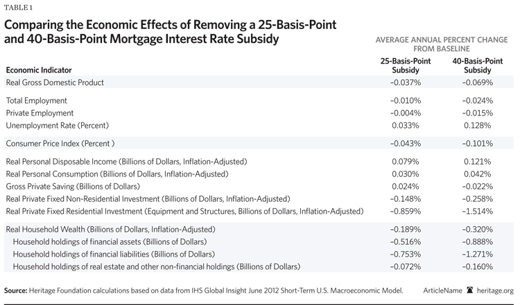
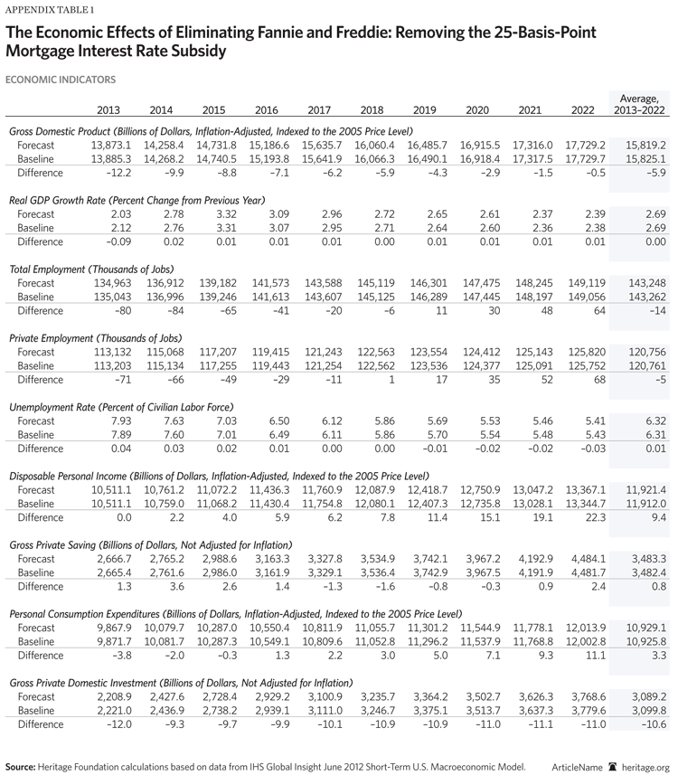
Winding down Fannie and Freddie by ceasing new activity in the mortgage market would have minimal and predictable effects on the U.S. economy. Relative to baseline levels, real (inflation-adjusted) gross domestic product (GDP) declines an average of $6 billion per year over the 10-year forecast period. To put this economic outcome in broad context, the average baseline level of the real economy is $15.8 trillion over the 10-year forecast period, so the impact on the economy over the 10-year forecast is less than 0.037 percent.[5]

Employment. As the real non-housing, nongovernment economy improves relative to the baseline for the 10-year forecast, the labor market stabilizes. The slight slowdown in real output would push down total employment on average 14,000 jobs (0.01 percent) per year and private employment 5,000 jobs (0.004 percent) per year relative to baseline levels. The decrease in the mortgage and housing markets would translate to an average 3,200 (0.43 percent) fewer jobs per year in the construction sector relative to baseline levels. The differences, however, are minuscule relative to the overall labor market—the average level of total employment at baseline is 143 million jobs.

Household Income and Consumption. Real personal consumption declines slightly in the first few years of the forecast period, lagging behind the change in real personal income and real disposable income levels.[6] Real personal income levels trend positive beyond the first few years of the forecast period, driven in part by changes in nominal (not adjusted for inflation) personal interest income.[7] Real disposable incomes would increase on average $11 billion (0.08 percent) per year over the 10-year forecast. Real household personal consumption increases on average $3.2 billion (0.03 percent) per year relative to baseline levels.

Mortgages and Household Deleveraging. The composition of aggregate U.S. household portfolio holdings changes relative to the baseline due to the movement in borrowing and saving costs in the economy. Nominal household financial liabilities decline an average $124 billion (0.753 percent) per year over the 10-year period. The level of household financial assets (nominal) declines an average $281 billion (0.51 percent) per year relative to baseline levels. Household holdings of real estate and other nonfinancial assets decline an average $28 billion (0.072 percent) per year relative to baseline levels.

The cost of mortgage borrowing rises relative to other interest rates, which results in a substitution away from financial leverage in the economy. Home mortgage acquisitions fall an average $10 billion (2 percent) per year relative to baseline levels. Total home mortgages outstanding decline an average $87 billion (0.69 percent) per year over the 10-year forecast.

Homeownership. The rate of homeownership declines on average 0.112 percent over the 10-year period. The policy reform likely leads to tighter credit conditions, which—all else constant—would reduce home sales and thus homeownership, partly as a function of home sales. However, all else is not constant. Changes in other factors that are correlated with home sales, such as the price of homes and disposable incomes, could reduce the effect of the policy reform.

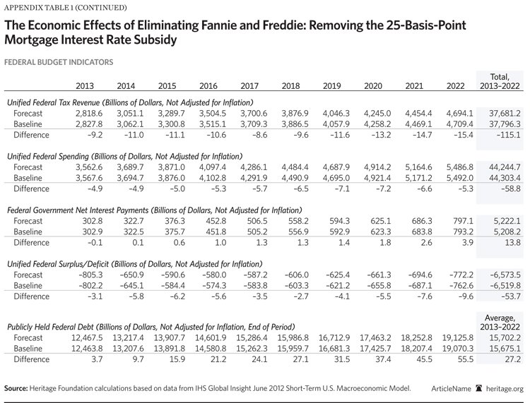
Cost to Taxpayers. Winding down GSE activity could push federal publicly held debt above baseline levels on average $27 billion (0.17 percent) per year relative to baseline levels. This dynamic result compares with the direct costs to the federal taxpayer of more than $150 billion since the 2008 takeover of Fannie Mae and Freddie Mac. The total GSEs' losses will cost the federal taxpayers an estimated $200 billion to $400 billion.[8]

The remainder of this report is structured as follows: Section 2 gives a brief overview of the housing GSEs and their relationship with the U.S. housing and mortgage markets. Section 3 gives an overview of the economic dynamics of the U.S. housing and mortgage markets. Section 4 presents and analyzes the dynamic simulation of the liquidation of the GSEs from the U.S. housing and mortgage markets. Section 5 is the conclusion.

Fannie Mae, Freddie Mac, and the U.S. Housing Market

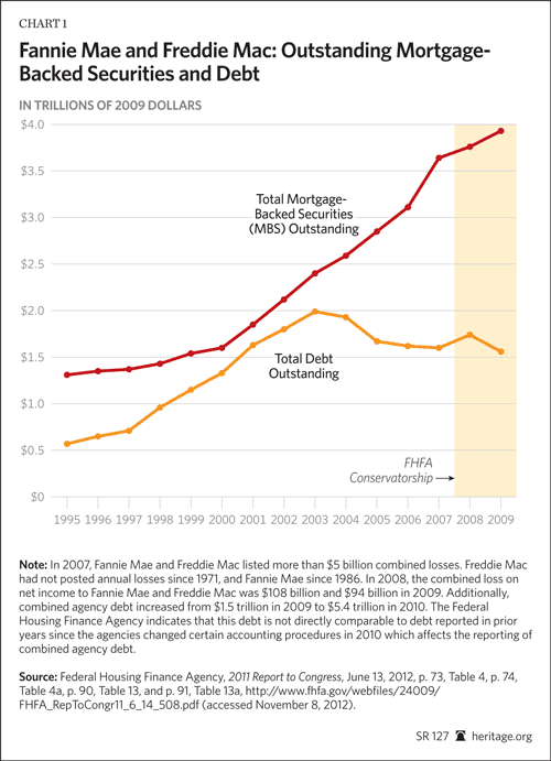
The housing GSEs have grown significantly in size and scope in the U.S. mortgage market since their origination. Fannie Mae was originally chartered in 1938 as the National Mortgage Association of Washington, and Freddie Mac was created in 1970.[9] Their asset holdings—either through mortgage securitizations or direct portfolio holdings—have increased from approximately 7 percent of total residential mortgage market originations in 1980 ($78 billion) to about 47 percent in 2003 ($3.6 trillion).[10]

By 2010, Fannie and Freddie owned or guaranteed approximately half of all outstanding mortgages in the United States, including a significant share of sub-prime mortgages, and they financed 63 percent of new mortgages originated that year.[11] Other federal agencies, including the Federal Housing Administration and the U.S. Department of Veterans Affairs, insured another 23 percent of home loans. This means that federal taxpayers guaranteed approximately 86 percent of all new mortgage originations in 2010.[12]

Outstanding Mortagebacked Securities and debt

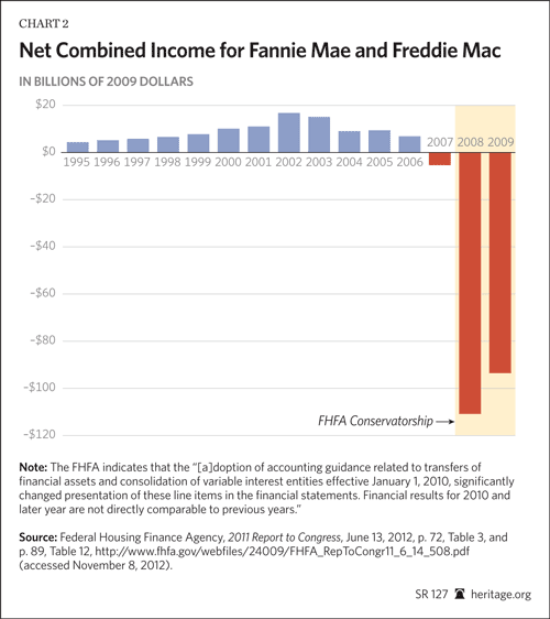
Fannie and Freddie were placed into conservatorship in 2008 to ensure they had the necessary capital to cover losses on the defaulted mortgage assets in their portfolios.[13] The federal take over has directly cost the federal taxpayer about $180 billion through March 2011, and the federal taxpayer could lose an additional $221 billion to $363 billion.[14] (See Chart 2.)

Net combined income for fannie mae and freddie mac

GSE interest rate subsidy

Fannie Mae and Freddie Mac, the mortgage government-sponsored enterprises (GSEs), are for-profit institutions operating under congressionally mandated missions to expand mortgage credit to specific income groups and achieve specific housing goals. Since 2008, Fannie Mae and Freddie Mac reside under the conservatorship of the Federal Housing Finance Agency (FHFA), and the agency debt and other mortgage-related holdings are directly guaranteed by the federal government.[15]

Securities held for investment

Prior to FHFA conservatorship and the explicit backing of the federal government, market purchasers of the GSE debt believed that Fannie Mae and Freddie Mac's agency debt was implicitly backed by the federal government. This belief stemmed from the many borrowing, tax, and regulatory advantages not conferred to any other shareholderowned corporation, including an official line of credit with the U.S. Treasury.[16] First, Fannie Mae and Freddie Mac were exempt from state and local income taxation. Second, they were exempt from Securities and Exchange Commission registration and bank regulations on security holdings. Third, they held a direct line of credit with the U.S. Treasury, issuing agency debt and borrowing between corporate AAA credit interest rate yields and U.S. Treasury interest rate yields.[17] Last, they received U.S. agency status and the guarantee of the federal government on mortgagebacked securities.

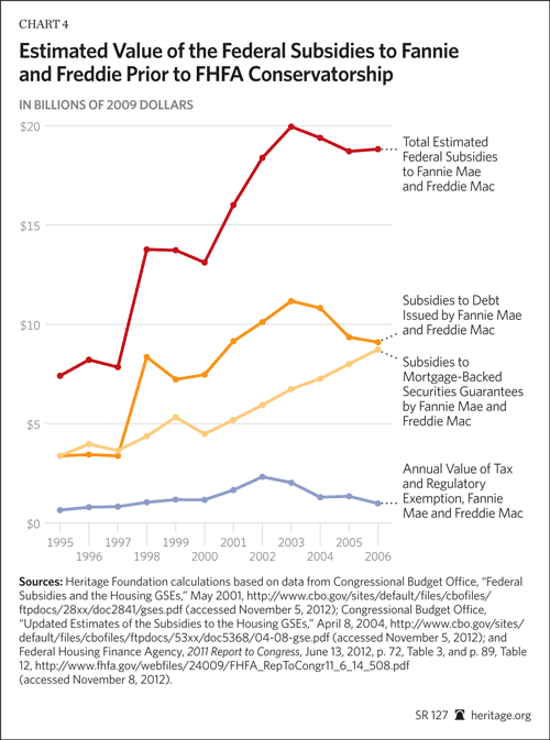
The annual estimated value of these subsidy benefits is substantial, ranging from about $7 billion to $20 billion before FHFA conservatorship. (See Chart 4.)

estimated value of the federal subsidies to Fannie and Freddie

Economists have made several attempts to estimate the value of these federal subsidies.[18] The Congressional Budget Office estimates the "agency debt" subsidy (lower borrowing costs) results in a 41 basis point value to shareholders and borrowers. Fannie Mae and Freddie Mac pass through 25 basis points of the subsidy value to borrowers and its shareholders retain an estimated 16 basis points on each dollar of debt. They estimate a subsidy value on mortgage-backed securities at 30 basis points, where 25 basis points are passed to the borrowers.[19]

Passmore, Sherlund, and Burgess estimate a 40 basis point subsidy to GSE debt and conclude a portion of this subsidy is passed to mortgage borrowers. They estimate that the pass-through of the GSE debt subsidy lowers mortgage rates to homeowners by 7 basis points, or 16 percent of the total 40 basis point subsidy value.[20] Ambrose and Warga estimate the interest rate subsidy toward the lower bound over AA-rated banking-sector bonds (20-29 basis points) and upper bound over AAA-rated bankingsector bonds (43-47 basis points).[21] Kauffman posits that Fannie Mae and Freddie Mac activity resulted in about a 10 basis point spread between the jumbo and conforming interest rates.[22]

Do the GSEs' contributions to a more efficient home mortgage market justify their special privileges? Because of their sheer size, dominance in the U.S. mortgage market, and special borrowing privilege with the U.S. Treasury, Fannie and Freddie have arguably held mortgage interest rates lower by an estimated 20 to 50 basis points.[23] The GSEs do not make failures in the U.S. housing and housing finance markets less likely.[24] Nor is it certain they have an intrinsic market efficiency advantage over other private mortgage underwriters.[25] Rather, the housing GSEs have likely expanded because of the advantage of the low-cost funding[26]—due to the implicit (now explicit) federal government guarantee—and federal government charters.[27]

One of Fannie and Freddie's federal charters or goals over the past two decades has been to expand U.S. homeownership.[28] While there may be some potential benefit to homeownership in the U.S.,[29] using the GSEs to achieve these policy goals is likely an inefficient, risky, and costly way to promote such societal benefits.[30] Congressional testimony shows that banks and lending institutions warned federal policymakers that achieving such outcomes would require departing from more prudent lending standards.[31] Indeed, the housing GSEs attempted to achieve this federal charter by expanding mortgage credit to a substantial share of sub-prime borrowers, which induced a stronger demand for mortgages over time.[32]

What does this mean for federal housing policy? Economists are still debating the causal role that Fannie and Freddie played in the recent housing bubble and the subsequent financial collapse of 2008. Despite this dispute, economists increasingly view the GSEs as a failed institutional model, which shielded them from losses due to their excessive risky behavior while allowing them to reap the rewards during periods of growth.[33]

The underwriting record of housing GSEs contains serious and systemic business and policy errors, and congressional leaders need to recognize the failure of this institutional model. Congressional leaders made the mistakes of creating Fannie and Freddie and subsidizing their activity in the U.S. mortgage market through special access to federal funds and an implicit guarantee.[34] They need to wind down Fannie and Freddie and free the U.S. housing market from the distortions that these institutions create.[35]

Dynamics in U.S. Housing and Mortgage Markets

The housing and mortgage markets affect the overall economy through many macroeconomic channels. For example, households generally treat housing and real estate as both an investment good and a consumption good. Indeed, U.S. households hold a substantial share of their overall asset portfolio in the housing and real estate markets.[36] The composition of total wealth is not the same across U.S. households. Households in the upper-income quintile hold significantly less of their total wealth in housing than households in the lower-income quintiles do.[37]

Changes to the valuation of these assets affect household wealth, which can induce changes in the additional housing (and non-housing) consumption and investment. Numerous economists have estimated that rising household wealth induces demand for new consumption. In fact, this link between housing wealth and consumption is more robust than for other forms of wealth, such as wealth held in the stock market.[38]

This relationship is less robust in the opposite direction, suggesting that declines in housing wealth do not tend to reduce consumption.[39] Additionally, the relationship between housing wealth and consumption is likely asymmetric because younger households may have a higher likelihood than older households to consume out of (positive) changes in housing wealth.[40]

Price fluctuations in the housing market have a considerable effect on the valuation of housing assets.[41] Housing prices change due to both demand-side and supply-side factors. Historically, key determinants for housing demand in the U.S. are price expectations vis-à-vis home prices, income levels, and regional economic performance.[42] Income levels and regional macroeconomic conditions greatly affect both the supply and demand in housing and mortgage markets at the national aggregate level.[43]

Nominal national home prices increased for three decades until 2006.[44] Real (adjusted for inflation) national home prices are more cyclical and have experienced several periods of ups and downs since the 1970s.[45] Regional home prices have followed a different pattern than nominal and real prices at the national level.[46]

House prices are volatile relative to observable changes in fundamentals. Glaeser, Gyourko, and Saiz estimate a model of housing bubbles that predicts that places with more elastic housing supply have fewer bubbles and shorter bubbles, with smaller price increases.[47] Housing supply at the national level looks relatively inelastic, but some regional housing markets have much more elastic housing supplies.[48] In many regional markets, the ratio of home prices to per capita income[49] rose dramatically from 2000 to 2005.[50] Homeowners had strong expectations of future price appreciation.[51]

From 2000 to 2007, there was a combination of a low interest rate policy[52] and an easing of lending standards in the U.S. housing and mortgage markets. Mortgage providers began to loosen lending standards even more than during the 1990s.[53] The GSEs were not exempt from the loosening of home mortgage lending standards.[54] The level of GSE activity increased substantially, whether through direct holdings or securitization.[55] During the 1990s, the GSE share of mortgage loans with high loan-to-value (LTV) ratios rose from around 6 percent of purchases in 1992 to 19 percent of purchases in 1995.[56] By 2007, Fannie and Freddie held "as much as 25 percent of its total loans with LTV above 80 percent and 18 percent with FICO scores below 660."[57]

During the boom period (2002-2006), debt-to-income levels rose sharply for many U.S. households. Mortgage and non-home-related debt rose at a similar pace from 1996 to 2002, but mortgage-related debt accelerated faster than non-home-related debt accelerated from 2002 to 2005[58] While housing-related asset valuations were rising, the level of borrowing activity against the higher home values—home-equity-based mortgage borrowing—also increased.[59] This borrowing behavior remained mostly concentrated among younger households and households with low credit scores, and high initial credit card utilization rates contributed the most to this type of borrowing behavior.[60] From 2006 to 2008, home-equity-based borrowing accounted for a sizeable share of new mortgage defaults.[61]

Since 2006, national home prices have declined substantially, and some regional markets experienced catastrophic decreases. In many regional housing markets during the past couple of years, these price changes and weakening macroeconomic fundamentals (e.g., high unemployment rates and falling household incomes) have put downward pressure on both the demand and the supply of housing and mortgages.[62] The combination of dramatic asset price reversion and macroeconomic instability left—and still leaves—many households unable to stay current on their home payments. Consequently, beginning in 2006, the rate of defaults and delinquencies spiked as prices began to plummet.[63]

Because of the broad reach of the mortgage assets—including direct mortgage holdings and securitizations—to U.S. financial markets,[64] the recent downturn in prices dramatically affected the household wealth.[65] The loss of value in mortgage-related assets significantly affected financial institutions, especially Fannie and Freddie, which were systematically part of the financial system.

The Economic Effects of Fannie and Freddie Reform

In this section, we focus on a dynamic simulation of winding down the housing GSEs and their activity in the U.S. mortgage market. We first give an overview of the macroeconomic simulation and why we employed the GII structural model to study the overall policy question. We then discuss the results of the dynamic simulation.

Macroeconomic Simulation. The GII Short-Term Quarterly Economic Model is a broad, structural model of the U.S. economy with multiple macroeconomic channels that can be used to address the overall policy question relating to the liquidation of Fannie and Freddie. The dynamic simulation of this policy change largely concentrates on the particular macroeconomic channels relating to the potential changes to mortgage interest rates and mortgage terms.[66]

The GII model offers several advantages in addressing this policy question. First, the model consists of robust economic relationships, whether explicit or implicit, based on historical data. Second, we can estimate the general equilibrium effects of the policy change because the model accounts for feedback effects across multiple economic sectors. That is, the model determines the effects that direct shocks to one set of economic series will have on other series in the model. Thus, the model determines the dynamic effects that changes on direct levers (e.g., interest rate shocks) would likely have on indirect channels in the model (e.g., household incomes, the affordability of homes, and changes to household wealth).

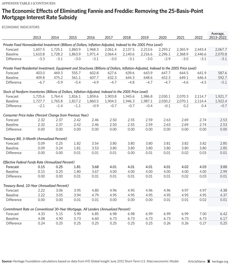
Additionally, since this counterfactual experiment compares an economy with Fannie and Freddie with an economy without these GSEs, we ran two simulations to test the sensitivity of the GII model to the 25 basis points assumption. The first simulation assumed the same 25 basis point change in the mortgage commitment rate, and we turned off the Federal Reserve reaction function in the GII model. The second simulation assumed a 40 basis point change in the mortgage commitment rate. Appendix Tables 2 and 3 in Appendix B present the results of these two sensitivity simulation runs.

Results of Dynamic Simulation. The U.S. economy is stable in general equilibrium as the policy change of winding down and eliminating the housing GSEs unfolds. In broad context, the overall economy-wide effect is minimal relative to average baseline levels of real GDP ($15.8 trillion). Eliminating the housing GSEs could push the real economy an average of $9 billion below the baseline over the five-year forecast and $6 billion (0.037 percent) per year below the baseline for the 10-year forecast. The non-housing, nongovernment real economy could fall an average of $3 billion below the baseline for the five-year forecast and an average $2 billion below the baseline for the 10-year forecast. These differences in real output are minuscule compared with the overall economy in the forecast period.

The change in real output over the 10-year forecast period would push total employment baseline levels on average 14,000 jobs (0.01 percent) per year. As the labor market stabilizes over the 10-year forecast period, private employment would decrease only 5,000 jobs (0.004 percent) per year relative to baseline levels[67] Additionally, as households take less leverage positions in the U.S., particularly in housing-related consumption, construction-related employment slightly slows by an average of 3,200 (0.43 percent) fewer jobs per year over the 10-year forecast.[68]

The results indicate that household balance sheets improve as real disposable income grows and as spending on durable and non-durable (non-housing) commodities rises. Real personal consumption declines in the first few years, lagging behind the change in real personal income and real disposable income levels. Over the 10-year forecast, real disposable income grows an average of $9 billion (0.079 percent) per year, and real consumption of durable and non-durable goods and services rises $3 billion (0.03 percent) per year relative to baseline levels.

Real personal income levels trend positive beyond the first few years of the forecast horizon largely because of changes in the nominal personal interest income. Nominal personal interest income increases an average of 1.2 percent relative to baseline levels in the five-year forecast period and 1.6 percent relative to baseline levels over the 10-year forecast period. The change in personal interest income is largely driven by changes to a basket of interest rates. This composite of lagged interest rates in the model increases an average of 10 basis points per year to baseline levels over the 10-year forecast period.[69]

As borrowing costs rise, particularly for mortgages, households reduce the amount of housing leverage they hold. Gross private savings increase on average $820 million (0.024 percent) per year relative to baseline levels, and the nominal level of household holdings of financial liabilities declines an average $126 billion (0.75 percent) per year relative to baseline levels.[70] While households reduce their financial debt levels, their holdings of other financial and non-financial assets decline relative to the baseline.[71] Nominal household holdings of financial assets decline 0.52 percent, and holdings of real estate and other non-financial assets decline 0.07 percent.[72] As a result, real household net worth[73] declines an average of 0.19 percent relative to the baseline for the 10-year forecast.

The change in household net worth is an aggregate measure in the GII model and thus does not indicate the relative change between households at different income levels. Wealthier households could likely benefit more from the GSE subsidy than less wealthy households benefit. Without the GSE subsidy, wealthier households have a stronger financial incentive to reduce holdings of both mortgage debt and bond holdings. (See Text Box: Changes in Household Wealth.) Lower wealth households are less likely to hold both mortgage debt and bonds, so a larger portion of the changes to aggregate household net worth likely occurs in wealthier households.

Who Benefits from Changes in Household Wealth?

A crucial question is which households are better off or worse off because of the policy change. Additionally, given a steady-state income—a state in which the economy has converged to equilibrium—would someone prefer to start life in an economy with or without the subsidy. The GII model is limited in its ability to answer these types of welfare questions. We can primarily gain insight to the aggregate changes in household wealth over the forecast frame. Thus, the findings in this study do not give insight into the relative changes in household wealth within income groups.

In a different dynamic general equilibrium framework, Jeske, Krueger, and Mitman find that removing the GSE subsidy would likely widen the gap between the median and average wealth measure. They estimate that the Gini coefficient for (net) wealth would increase 0.67 percentage point. Thus, when comparing stationary wealth distributions between an economy with the GSE subsidy and without the GSE subsidy, they find that removing the subsidy may lead to higher wealth inequality.[74]

In addressing the second question, they find that the welfare gains of the subsidy are monotonically increasing in wealth. Thus, in the hypothetical in which there is a choice to start in an economy without such a subsidy, lower-income households would likely benefit without the subsidy while households with high wealth would benefit from the subsidy. The rationale for this is:

[T]he subsidy keeps interest rates on the financial assets of wealthy households high (since the subsidy fuels a stronger demand), and second, it provides these households (which invest [more] in bonds and leverage substantially in real estate) with a direct subsidy for this investment strategy. Poorer households, on the other hand, derive a large share of their current resources from labor income which is subject to the tax that finances the mortgage interest rate subsidy. Thus these households would prefer having the subsidy and the tax that comes with it removed, especially if their wealth is so low that debtfinanced investment into real estate becomes suboptimal for them and thus the subsidy does not apply to these households.[75]

Comparing Interest rate Subsidy

Comparing Interest rate Subsidy

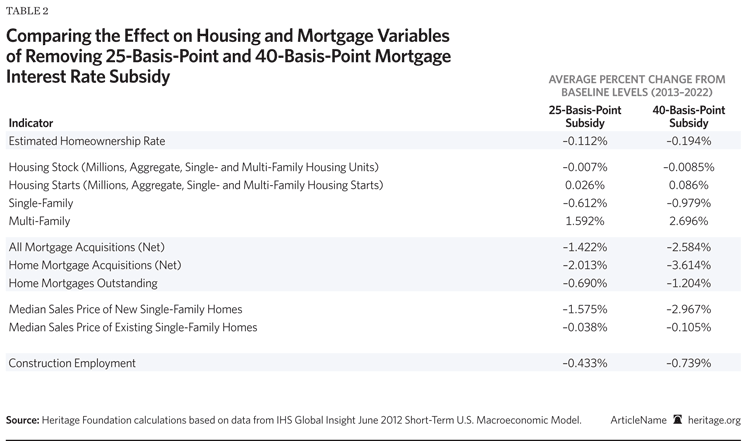
As households respond to the higher borrowing costs in mortgage markets, the level of housing-related and mortgage-related debt declines in the U.S. economy. Total mortgage acquisitions fall roughly 1.42 percent relative to baseline levels, home mortgage acquisitions fall 2.01 percent, and total home mortgages outstanding decline by approximately 0.69 percent.[76] The U.S. housing stock[77] and housing starts experience negligible changes: U.S. housing stock (single-family and multi-family), excluding stock of mobile home units, decreases an average of 0.007 percent relative to the baseline, while housing starts (single-family and multi-family) increase slightly by 0.026 percent.[78]

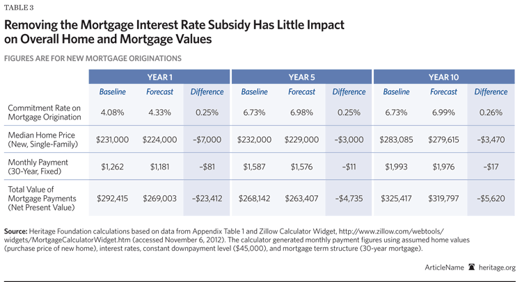
There is little inflationary pressure in the economy. The year-to-year Consumer Price Index (CPI) changes fall relative to the baseline, and prices begin to rise above the baseline beginning in year 2019. Home prices are also stable over the forecast period. Over the 10-year forecast period, the median price of new single-family homes falls an average of 1.58 percent, while the median price of existing single-family homes declines 0.04 percent.[79] Even a modest decrease in median home prices on existing or new single-family homes should not necessarily matter. If households are making housing-related consumption decisions with lower leverage (debt) positions, then—economically speaking—the slight decrease over the forecast period in the price of these assets should not negatively impact them.

Impact on Home and Mortgage values

What is the likely impact of eliminating the housing GSEs on U.S. homeownership? Holding all else constant, tighter credit conditions (e.g., raising down-payment requirements) would likely reduce home sales and thus homeownership across the age distribution.[80] However, "all else" would not be held constant. This effect may be reduced by changes in other factors that correlate with home sales, such as the price of homes and disposable incomes. The simulation results indicate that U.S. sales of new homes would fall an average of 0.81 percent and sales of existing homes would fall 1.58 percent over the 10-year forecast period. The results suggest that real household incomes would rise over the forecast period and that the price of new and existing homes would fall slightly. Consequently, U.S. homeownership would decline negligibly by an average of 0.11 percent over the 10-year forecast period.

Federal Publicly Held Debt. Rising long-term interest rates push the interest payments on the federal debt higher. Eliminating the housing GSEs could push publicly held debt higher by an average of 0.17 percent relative to baseline levels over the 10-year forecast.

Eliminating GSE activity in the U.S. mortgage market would result in a minimal and predictable decline in the U.S. economy over the 10-year forecast. Beyond the first few years of the forecast period, as the real economy begins to improve, the U.S. labor market begins to stabilize.

Conclusion

After more than three decades of experience with boom and bust cycles in the housing market, which have affected not only household income and wealth but also financial markets, federal policymakers should seriously reconsider the federal government's role in shaping housing policy. Fannie Mae and Freddie Mac distort the U.S. housing and mortgage market at substantial risk to households and U.S. taxpayers.

The estimates in this report provide additional evidence that the housing GSEs should not be a part of the path to a new housing market and economy. Ceasing new GSE activity would remove a subsidy in the mortgage market—a subsidy that has induced households to take on more debt-related consumption, including in many households that were never in a position to handle the mortgage debt.

The policy reform would have little impact on the overall housing market over the 10-year forecast period. The overall impact on U.S. homeownership is predictable and minimal because the policy reform has little impact on the U.S. economy in the long run. Over the entire 10-year forecast period, the impact on household balance sheets is minimal and predictable resulting in a stabilized labor market and real economy.

Appendix A: Methodology

Overview of the IHS Global Insight Quarterly Model of the U.S. Economy

CDA analysts used the IHS Global Insight 2012 June Quarterly Short-Term Model of the U.S. economy to estimate the overall net economic effects of gradually liquidating Fannie and Freddie. The baseline forecast is the forecast of the economic future with the housing Government-Sponsored Enterprises (GSEs), Fannie and Freddie, in existence.[81]

The IHS Global Insight Quarterly Short-term model is largely an econometrically estimated model of the U.S. economy that combines both demand-side and supply-side features. It is crucial, however, to keep in mind that all of the economic relationships, explicit and implicit, in the GII model as well as other empirical models of the U.S. housing market based on historical data assume the existence of the two housing finance GSEs.[82]

Simulating the Economic Effects of Liquidating Fannie and Freddie

Since the counterfactual experiment compares an economy with Fannie and Freddie with one without them, we run two simulations to test the sensitivity of the GII model to the 25 basis point assumption. The first sensitivity run assumes the same 25 basis point change in the mortgage commitment rate, and we turn off the lever in the GII model for the Federal Reserve reaction function. The second simulation assumes a 40 basis point change in the mortgage commitment rate and leaving the Federal Reserve reaction function turned on. See Appendix Table 2 and Appendix Table 3 in Appendix B for the results of these two sensitivity simulation runs.

To address these policy questions with the GII model, either the variable in question needs to explicitly exist in it or a relationship to a variable inside the model needs to be established using an outside model. Some model variables—those which are identities—cannot be used as levers in a simulation because changing them would invalidate the underlying econometric interrelationship of the entire model.

All changes were introduced to the model as immediate and permanent changes over the full 10-year forecast. Additionally, the changes were introduced in the model to the add-factor (the stochastic/error component) of the variable unless otherwise indicated.[83] Therefore, there is likely some adjustment to the variable over the 10-year forecast where the add-factor was overridden.

Because no variable in the GII model shows the asset valuation of GSE mortgages, the sizeable effect of this change would operate via the interest rates and conditions on mortgage lending. That is, if the GSEs are selling assets as a result of liquidation, then their price would fall, mortgage interest rates would rise, and mortgage lending conditions would likely change.[84]

A crucial question for modeling purposes would be whether these institutions are simply selling mortgages or whether they are also pulling out of the mortgage insurance business. If they are holding mortgages themselves, then this would push interest rates higher. However, if they are no longer providing mortgage insurance, then rates would likely rise by even more, and the lending terms and conditions in the private sector would tighten.[85] As a result, at least in the short run, higher rates and tighter lending conditions would induce change in demand for housing and mortgages, which would push prices (and likely activity) down.

Changes to Interest Rates on U.S. Residential Mortgages. One of the dominant policy channels in the simulation is the change in interest rates in the mortgage markets.[86] At a minimum, liquidating the housing GSEs would increase the cost of borrowing in the short run in the housing and mortgage markets of the U.S. economy. It is widely believed that eliminating the GSEs in the secondary mortgage markets will result in a change in the mortgage interest rate spread.[87] Without the GSE guarantees, mortgage holders—such as pension funds and banks—will want a higher interest rate to offset the increased risk of holding mortgages. The spread could be affected by changes in demand for Treasury securities (which are often an index for mortgages), the supply of Treasuries, or even views of the riskiness of the mortgages and other alternative financial products.

We assume that the impact will be an increase between 25 and 40 basis points.[88] and we assume an immediate and permanent cost of borrowing in the mortgage market. The IHS/Global Insight model has a series that captures the commitment rate on conventional 30-year mortgages (annualized rate and an aggregate of all lenders).[89] This variable is stochastic in the model; therefore, we make the change as an override to the stochastic component of the variable. It is important to note, however, that these levers may not capture potential volatility well. Without the GSEs, we could expect interruption in the supply of funds for mortgages. This could create large or frequent swings in the mortgage rate. We did not assume any exogenous change in volatility to the interest rate series in the model, including the commitment rate on conventional 30-year mortgages.

Estimated U.S. Homeownership Rate. The homeownership rate is not a variable in the model. However, homeownership is related to the number of homes sold, which is derived from the existing single-family home sales in the model. We used an OLS regression model to estimate homeownership as a function of existing single-family home sales (HU1ESOLD). We introduce this new variable into the GII model to generate projected homeownership rates (RHOMEOWNNS) based on the forecasted HU1ESOLD.[90]

Appendix B

Removing the 25 basis point mortgage interest rate subsidy

Removing the 25 basis point mortgage interest rate subsidy

Removing the 25 basis point mortgage interest rate subsidy

About the Authors

John L. Ligon is a Policy Analyst in the Center for Data Analysis at The Heritage Foundation.

William W. Beach is Director of the Center for Data Analysis, and Lazof Family Fellow in Economics, at The Heritage Foundation.

[1] The authors use "housing GSEs" and the nicknames Fannie Mae and Freddie Mac interchangeably in this report.

[2] The Heritage Foundation argues that Congress should eliminate Fannie and Freddie and remove any implicit or direct guarantee by federal taxpayers. For more details about this specific policy reform proposal, see David C. John, "Free the Housing Finance Market from Fannie Mae and Freddie Mac," Heritage Foundation Backgrounder No. 2577, July 12, 2011, http://www.heritage.org/research/reports/2011/07/free-the-housing-finance-market-from-fannie-mae-and-freddie-mac.

[3] For a discussion of the GII model and the authors' methodology, see Appendix A.

[4] This study investigates the counterfactual experiment in which no housing GSE (e.g., Fannie Mae and Freddie Mac) exists or distorts the U.S. housing finance system. The assumptions that relate to the effects on mortgage interest rates are implemented as immediate and permanent changes. Using a structural model with sufficient detail across multiple economic sectors is an appropriate model to complete this type of policy simulation. While alternate economic models (such as a standard input-output model) have certain strengths, simulations investigating long-run perturbations relative to trend requires sufficient economic detail. The GII model is robust in capturing the dynamic effects of changes in certain parts of the financial sector on other sectors of the economy. For the simulation details, see Appendix B.

[5] All results are expressed relative to the GII June Short-Term Model Baseline forecast of the economy. The baseline economic forecast assumes no change to the U.S. mortgage market and the housing GSEs remain in existence. For additional details, see Appendix B.

[6] The real economic indicators were adjusted for inflation using 2005 as the base year. Nominal indicators were not adjusted for inflation.

[7] Nominal personal interest income would increase an average of $16 billion per year relative to baseline in the five-year forecast period and an average of $30 billion per year over the 10-year forecast frame. A variable measuring the composite of lagged interest rates is a primary driver of this variable in the GII model. This variable increases an average of 7 basis points per year relative to baseline in the five-year frame and an average of 10 basis points per year in the 10-year frame.

[8] The Congressional Budget Office (CBO) estimated in 2010 that the total direct subsidy costs to Fannie Mae and Freddie Mac would equal $389 billion over the 10-year budget projection period. In a 2011 report, CBO analysts indicate the losses to federal taxpayers from November 2008 to the end of March 2011 totaled $154 billion in capital (net $24 billion in dividends on its preferred stock). Deborah Lucas, "The Budgetary Cost of Fannie Mae and Freddie Mac and Options for the Future Federal Role in the Secondary Mortgage Market," statement before the Committee on the Budget, U.S. House of Representatives, June 2, 2011, p. 2, http://www.cbo.gov/sites/default/files/cbofiles/ftpdocs/122xx/doc12213/06-02-gses_testimony.pdf (accessed June 4, 2012). See also Peter J. Wallison, Alex J. Pollock, and Edward J. Pinto, "Taking the Government Out of Housing Finance: Principles for Reforming the Housing Finance Market," American Enterprise Institute Policy White Paper, preliminary draft, January 20, 2011, p. 3, http://www.aei.org/files/2011/01/20/HousingFinance.pdf (accessed June 5, 2012).

[9] W. Scott Frame and Lawrence J. White, "Fussing and Fuming over Fannie and Freddie: How Much Smoke, How Much Fire?" Journal of Economic Perspectives, Vol. 19, No. 2 (Spring 2005), pp. 159–160.

[10] Ibid., p. 162.

[11] Lucas, "The Budgetary Cost of Fannie Mae and Freddie Mac," p. 7.

[12] Ibid., p. 7.

[13] The Housing and Economic Recovery Act (HERA) of 2008 conferred to the FHFA the power to place Fannie Mae and Freddie Mac in federal conservatorship, which the FHFA did in September 2008. Previously, Fannie Mae and Freddie Mac were regulated by the Office of Federal Housing Enterprise Oversight (OFHEO). HERA transferred the regulatory responsibility to the FHFA.

[14] The losses to federal taxpayers from November 2008 to the end of March 2011 totaled $154 billion in capital (net $24 billion in dividends on its preferred stock). Lucas, "The Budgetary Cost of Fannie Mae and Freddie Mac," p. 2, and Wallison et al., "Taking the Government out of Housing Finance," p. 3.

[15] The federal government provides direct financing since the 2008 conservatorship, and the agency debt is not considered official government debt and is not included in the accounting of federal publicly held debt. Moreover, the level of agency debt is massive, approaching the total value of U.S. Treasury debt. In 1970, this agency debt was 15 percent of Treasury debt; in 2010, agency debt was 81 percent ($7.5 trillion) of Treasury debt. Alex J. Pollack, "The Government's Four-Decade Financial Experiment," The American, July 13, 2011, http://www.american.com/archive/2011/july/the-government2019s-four-decade-financial-experiment (accessed June 4, 2012), and Viral V. Acharya et al., Guaranteed to Fail: Fannie Mae, Freddie Mac, and the Debacle of Mortgage Finance (Princeton, NJ: Princeton University Press, 2011), pp. 50–54.

[16] The mortgage GSEs, Fannie and Freddie, were exempt from many state investor protection laws. The GSEs also received specific federal charters, mainly issuances of mortgage credit to income-specific groups of households. Dwight M. Jaffee and John M. Quigley, "Housing Subsidies and Homeowners: What Role for Government-Sponsored Enterprises?" University of California, Berkeley, Institute of Business and Economic Research and Fisher Center for Real Estate and Urban Policy Working Paper No. W06-006, January 2007, pp. 120–123, http://urbanpolicy.berkeley.edu/pdf/JQ_Housing_Subsidies_Proof_053007.pdf (accessed November 8, 2012).

[17] Debt issued by Fannie Mae and Freddie Mac is considered "agency securities," and the debt is issued with interest rate yields between corporate (AAA) debt and the yields on U.S. Treasury obligations. Ibid., p. 122.

[18] Frame and White provide a comprehensive summary of the studies attempting to estimate the value of the of the GSE subsidy. Frame and White, "Fussing and Fuming over Fannie and Freddie," pp. 159–160.

[19] Congressional Budget Office, "Federal Subsidies and the Housing GSEs," May 2001, pp. 23 and 26–28, http://www.cbo.gov/sites/default/files/cbofiles/ftpdocs/28xx/doc2841/gses.pdf (accessed November 5, 2012). Douglas Holtz-Eakin, "Updated Estimates of the Subsidies to the Housing GSEs," letter to Senator Richard C. Shelby, Chairman, Committee on Banking, Housing, and Urban Affairs, U.S. Senate, April 8, 2004, http://www.cbo.gov/sites/default/files/cbofiles/ftpdocs/53xx/doc5368/04-08-gse.pdf (accessed November 5, 2012).

[20] Wayne Passmore, S. Sherlund, and G. Burgess, "The Effect of Housing Government Sponsored Enterprises on Mortgage Rates," Real Estate Economics, Vol. 33. No. 3 (2005), pp. 19–22.

[21] Brent Ambrose and Arthur Warga, "Measuring Potential GSE Funding Advantages," Journal of Real Estate Finance and Economics, Vol. 25. Nos. 2–3 (2002), pp. 129–150.

[22] Alex Kauffman, "The Influence of Fannie and Freddie on Mortgage Loan Terms," Board of Governors of the Federal Reserve Board, Divisions of Research and Statistics and Monetary Affairs, May 7, 2012, pp. 19–21, http://www.federalreserve.gov/pubs/feds/2012/201233/201233pap.pdf (accessed November 11, 2012).

[23] For an overview of the interest rate subsidy the GSEs create, see Appendix B. For partial dynamic simulation results of introducing higher borrowing rates to the market as a result of eliminating Fannie and Freddie from federal government guarantee, see Appendix B.

[24] Lawrence J. White, "The Way Forward: U.S. Residential Mortgage Finance in a Post-GSE World," March 3, 2011, pp. 11–13, http://web-docs.stern.nyu.edu/old_web/economics/docs/workingpapers/2011/white-residential%20mortgage%20finance%203.3.11.pdf (accessed November 5, 2012).

[25] Lawrence J. White, "Focusing on Fannie and Freddie: The Dilemmas of Reforming Housing Finance," Journal of Financial Services Research, Vol. 23, No. 1 (February 2003), pp. 50–53.

[26] White notes that GSEs have had lower capital requirements than other U.S. depository institutions (on whole loans)—2.5 percent versus 4 percent; required to hold only 0.45 percent capital against the credit risk of mortgage-backed securities (MBS) on which they issued guarantees; and even if U.S. depository institutions chose to hold these GSE MBSs in their portfolios, they were required to hold 1.6 percent capital instead of 4 percent. White, "The Way Forward," p. 14.

[27] Frame and White provide an overview of the GSEs' special privileges, which before they were taken into federal conservatorship included having a direct-line of credit with the U.S. Treasury. Frame and White, "Fussing and Fuming over Fannie and Freddie," pp. 160–165.

[28] Ibid., pp. 162–163.

[29] Numerous economists and policy experts across the ideological divide posit that there are likely positive externalities to homeownership, while acknowledging the GSEs likely represent an inherently inefficient, risky, and costly way to promote these benefits to society. The federal government creates strong incentives for new construction and housing consumption via the tax code, completely separate from policy vis-à-vis the GSEs. Frame and White note that "[the] largest incentives [to encouraging U.S. construction and housing consumption] pertain to income tax advantages: the exclusion of the implicit income from housing by owner-occupiers, while allowing the deduction of mortgage interest and local real estate taxes." See Frame and White, "Fussing and Fuming over Fannie and Freddie," p. 171, White, "Focusing on Fannie and Freddie," pp. 48–49, and Acharya et al., Guaranteed to Fail, pp. 167–172.

[30] When compared with other countries, the U.S. is not even in the top five among Organization for Economic Co-operation and Development (OECD) countries in homeownership rates. Acharya et al., Guaranteed to Fail, pp. 116–123.

[31] Edward J. Pinto, "GSE Affordable Housing Goals: Politicized Credit Allocation," American Enterprise Institute, January 5, 2011, p. 4, http://www.aei.org/files/2012/01/06/-gse-affordable-housing-goals-politicized-credit-allocation_093515477777.pdf (accessed June 4, 2012).

[32] Acharya et al., Guaranteed to Fail, pp. 45–60.

[33] Ibid., pp. 3–6.

[34] John, "Free the Housing Finance Market from Fannie Mae and Freddie Mac."

[35] Frame and White, "Fussing and Fuming over Fannie and Freddie," pp. 175–180. David John outlines a detailed plan to achieving a housing market free of Fannie and Freddie. John, "Free the Housing Finance Market from Fannie Mae and Freddie Mac." Moreover, various proposals would address the issue of Fannie and Freddie and the U.S. housing market. Most of these proposals stop short of eliminating the link of the federal government to these agencies. The Obama Administration has advanced policy options in which they discuss potential changes to the structure of these agencies, yet they fail to offer one specific approach. See U.S. Department of Treasury and U.S. Department of Housing and Urban Development, "Reforming America's Housing Financial Market: A Report to Congress," February 2011, http://portal.hud.gov/hudportal/documents/huddoc?id=housingfinmarketreform.pdf (accessed October 23, 2012).

[36] Per Yi and Lang, the share of households' total assets represented in housing assets has fluctuated substantially over the past few decades. This share was around 20 percent in the mid-1960s and around 27 percent in the mid-1980s. The share was approximately 20 percent in 2000 and then rose to 30 percent by 2004 before dropping to around 25 percent in 2008. Flavin and Yamashita estimate that households between the ages of 18 and 30 hold roughly 68 percent of their total wealth in housing-related assets. The ratio of housing-related assets to household net worth declines as households' age. Additionally, households finance a significant share of their housing and real estate holdings with mortgage-related debt. Flavin and Yamashita also estimate that households ages 18 to 20 years hold mortgages with principal value at roughly 280 percent of total net wealth. Their estimates indicate that this ratio falls to 0.038 for households age 71 years and older. In other words, the principal value of mortgages held falls to less than 4 percent of total net wealth. Wenli Li and Fang Yang, "American Dream or American Obsession? The Economic Benefits and Costs of Homeownership," Federal Reserve Bank of Philadelphia Business Review, Quarter 3, 2010, http://www.philadelphiafed.org/research-and-data/publications/business-review/2010/q3/brq310_benefits-and-costs-of-homeownership.pdf (accessed October 23, 2012), and Majorie Flavin and Takashi Yamashita, "Owner-Occupied Housing and the Composition of the Household Portfolio," American Economic Review, Vol. 92, No. 1 (March 2002), p. 352.

[37] Diaz and Luengo-Prado find a high level of inequality in the wealth composition across U.S. households. Using a dynamic general equilibrium framework, they find that "households in the top 20% of the wealth distribution hold 56.4% of all residential assets and 98.9% of all financial assets; and housing wealth represents 96.3% of total wealth for households in the bottom 80% of the wealth distribution, whereas this proportion goes down to 26.8% for households in the top 20%." Antonia Diaz and Maria Jose Luengo-Prado, "The Wealth Distribution with Durable Goods," International Economic Review, Vol. 51, No. 1 (February 2010), pp. 143–170.

[38] Karl E. Case, John M. Quigley, and Robert J. Shiller, "Comparing Wealth Effects: The Stock Market vs. the Housing Market," Advances in Macroeconomics, Vol. 5, No. 1 (2005), pp. 1–34, http://www.econ.yale.edu/~shiller/pubs/p1181.pdf (accessed June 4, 2012), and Raphael Bostic, Stuart Gabriel, and Gary Painter, "Housing Wealth, Financial Wealth, and Consumption: New Evidence from Micro Data," University of Southern California, December 2005.

[39] Case et al., "Comparing Wealth Effects," p. 25.

[40] Gary V. Engelhardt, "House Prices and Home Owner Saving Behavior," Regional Science and Urban Economics, Vol. 26, Nos. 3–4 (June 1996), pp. 313–336. Kennickell and Lusardi estimate that about 8 percent of total wealth holdings arise from precautionary savings. While this accounts for a small amount of wealth, this motive is more important to older households and business owners than young and middle-aged households. Arthur Kennickell and Annamaria Lusardi, "Disentangling the Importance of the Precautionary Saving Motive," National Bureau of Economic Research Working Paper No. 10888, November 2004, http://www.nber.org/papers/w10888.pdf?new_window=1 (accessed January 2, 2013).

[41] Nakajima gives a comprehensive overview of house price dynamics in the U.S. and develops a theory of house prices on the equivalence between user costs and rents. The model indicates that expectations explain much of the change in the trend in house price behavior. Makoto Nakajima, "Understanding House-Price Dynamics," Federal Reserve Bank of Philadelphia Business Review, Quarter 2, 2011, http://www.phil.frb.org/phil_mailing_list/research-and-data/publications/business-review/2011/q2/brq211_understanding-house-price-dynamics.pdf (accessed June 14, 2012).

[42] There has been substantial price dispersion over the past few decades and across different regions of the U.S. Glaeser, Gyourko, and Saks suggest that the regional variation in price behavior and changes to key supply indicators resulted more from changes in the regulatory environment affecting housing supply. Edward L. Glaeser, Joseph Gyourko, and Raven E. Saks, "Why Have Housing Prices Gone Up?" Harvard Institute of Economic Research Discussion Paper No. 2061, February 2005, at http://ssrn.com/abstract=658324 (accessed June 11, 2012).

[43] Min Hwang and John M. Quigley, "Economic Fundamentals in Local Housing Markets: Evidence from U.S. Metropolitan Regions," Journal of Regional Science, Vol. 46, No. 3 (August 2006), pp. 425–453, and Karl E. Case and John M. Quigley, "How Housing Busts End: Home Prices, User Cost, and Rigidities During Down Cycles," University of California, Berkeley, Institute of Business and Economic Research, Program on Housing and Urban Policy Working Paper No. W08-008, September 1, 2009, pp. 460–466 and 467–471, http://escholarship.org/uc/item/6mh9m4ff.pdf (accessed November 5, 2012).

[44] Case and Quigley, "How Housing Busts End," pp. 477–479.

[45] Ibid. Case and Quigley summarize the nominal changes to gross residential investment, gross domestic product, and housing starts during four down cycles in the U.S. housing market from 1973 to 2008. The authors note four down cycles by quarter: 1973 Q1 (peak) to 1975 Q1 (trough); 1978 Q3 (peak) to 1982 Q3 (trough); 1986 Q4 (peak) to 1991 Q1 (trough); and 2006 Q1 (peak) to 2007 Q4 (trough). Interest rate policies aimed to reduce inflationary pressures in the economy induced the first three down cycles, especially in 1974–1975 and in 1980–1982. Karl E. Case and John M. Quigley, "How Housing Booms Unwind: Income Effects, Wealth Effects, and Feedbacks Through Financial Markets," European Journal of Housing Policy, Vol. 8, No. 2 (June 2008), p. 173.

[46] Case and Quigley, "How Housing Busts End."

[47] Edward L. Glaeser, Joseph Gyourko, and Albert Saiz, "Housing Supply and Housing Bubbles," National Bureau of Economic Research Working Paper No. 14193, July 2008, p. 28, http://www.nber.org/papers/w14193 (accessed November 27, 2012).

[48] House prices are generally volatile relative to observable changes in economic fundamentals, especially regional economic fundamentals. Glaesar, Gyourko, and Saiz estimated a model of housing bubbles that predicts that places with more elastic housing supplies have fewer bubbles and shorter bubbles with smaller price increases. Glaeser et al., "Housing Supply and Housing Bubbles," pp. 19–20. For a comprehensive overview of the most recent housing bubble, see Adam J. Levitin and Susan M. Wachter, "Explaining the Housing Bubble," September 1, 2010, revised May 16, 2012, http://papers.ssrn.com/sol3/papers.cfm?abstract_id=1669401 (accessed June 4, 2012).

[49] Income is a key determinant of effective final demand in the housing market. Karl E. Case, John M. Quigley, and Robert J. Shiller, "Home-Buyers, Housing and the Macroeconomy," University of California, Berkeley, Institute of Business and Economic Research, Program on Housing and Urban Policy Working Paper No. W04-004, November 18, 2003, pp. 152–156, http://escholarship.org/uc/item/0v59r392 (accessed June 4, 2012). The level of volatility in income matters in guiding housing consumption. Diaz and Luengo-Prado show in a dynamic general equilibrium framework that "current earnings are a good indicator of permanent income (which guides housing purchases) with persistent earnings but not with volatile earnings." Diaz and Luengo-Prado, "The Wealth Distribution with Durable Goods," p. 167.

[50] The ratio of home prices to per capita income from 1985 to 2002 has been relatively stable in 43 states. In the eight other states, this ratio has been quite cyclical and volatile. Case et al., "Home-Buyers, Housing, and the Macroeconomy," pp. 151–156.

[51] Case et al., "Home-Buyers, Housing and the Macroeconomy," and Edward L. Glaeser, Joshua D. Gottlieb, and Joseph Gyourko, "Can Cheap Credit Explain the Housing Boom?" National Bureau of Economic Research Working Paper No. 16230, July 2010, http://www.nber.org/papers/w16230 (accessed November 5, 2012).

[52] The inflation-adjusted yield on 10-year Treasury notes fell 120 basis points from 1996 to 2006, and 190 basis points from 2000 to 2005. Glaeser et al., "Can Cheap Credit Explain the Housing Boom?" Additionally, there is debate about the role that interest rates play in the pattern of home prices in the lead-up to the price peak of 2006. Numerous economists acknowledge that interest rate policy was one of many factors that drove the most recent housing bubble. See John B. Taylor, "Housing and Monetary Policy," National Bureau of Economic Research Working Paper No. 13682, December 2007, http://www.nber.org/papers/w13682 (accessed June 4, 2012); Case and Quigley, "How Housing Busts End"; and Levitin and Wachter, "Explaining the Housing Bubble." Some posit that interest rate policy can substantially affect price movements during bubble periods, particularly the bubble of 2000–2005. Charles Himmelberg, Christopher Mayer, and Todd Sinai, "Assessing High House Prices: Bubbles, Fundamentals, and Misperceptions," Journal of Economic Perspectives, Vol. 19, No. 4 (Fall 2005), pp. 67–92, http://pubs.aeaweb.org/doi/pdfplus/10.1257/089533005775196769 (accessed November 6, 2012), and Taylor, "Housing and Monetary Policy." Case and Quigley make the case that expansionary monetary policy by the Federal Reserve induced strong demand pressures in the U.S. mortgage and housing markets, beginning in 2002 with a strong demand for refinancing. Case and Quigley, "How Housing Busts End." Still, others argue that interest rates have little role and that other factors, such as price expectations of homeowners, matter more in the strong price movement during bubble periods. Glaeser et al., "Can Cheap Credit Explain the Housing Boom?" Additionally, Fannie and Freddie pass a substantial interest rate subsidy in the mortgage market due to their low-cost borrowing advantage with the Treasury. Taylor, "Housing and Monetary Policy"; Case and Quigley, "How Housing Busts End"; Levitin and Wachter, "Explaining the Housing Bubble"; Himmelberg et al., "Assessing High House Prices"; and Glaeser et al., "Can Cheap Credit Explain the Housing Boom?"

[53] Case, Glaeser, and Parker put forward that over the past decade, "[the] sum of outstanding mortgages with some form of mortgage insurance or guarantee (from the Federal Housing Administration or Veterans Administration, or through private mortgage insurance), the risk-tranched securities of Fannie Mae and Freddie Mac, and the subprime market has increased from 16 percent to just under 40 percent of total mortgage credit." Karl E. Case, "Real Estate and the Macroeconomy," Brookings Papers on Economic Activity, 2000, pp. 119-162, http://www.brookings.edu/~/media/Projects/BPEA/Fall%202000/2000b_bpea_case.PDF (accessed November 6, 2012).

[54] Acharya et al. note that the GSE affordable housing goals, particularly from 2003 to 2007, remained tied to a percentage of the total mortgage share—and not to particular growth targets. What did change substantially during this period was the GSE guarantee business in the mortgage-backed securities market. Acharya et al., Guaranteed to Fail, pp. 333-340.

[55] Gabriel and Rosenthal estimate substantial crowd-out effect in the U.S. mortgage market from 2004 to 2006 due to GSE activity. Their empirical estimates use data from the early 1990s, and they find little crowd-out effect from 1994 to 2003. Stuart A. Gabriel and Stuart S. Rosenthal, "Do the GSEs Expand the Supply of Mortgage Credit? New Evidence of Crowd Out in the Secondary Mortgage Market" May 27, 2010, http://ssrn.com/abstract=1760199 (accessed June 4, 2012).

[56] Glaeser, Gottlieb, and Gyourko argue that LTVs—essentially a measure of down-payment requirement levels on home purchase—were not a significant factor in the asset price appreciation during the 2000–2006 bubble and that there has been little variation in LTVs over time. These authors use data from 1998 to 2008. They do not control for changes in the sample of borrowers (borrower characteristics of particular concern), yet they acknowledge that these changes may be important "because we do know the number of buyers changed substantially over time: it nearly doubled from 1998–2005, before falling by over half between 2005 and 2008." Glaeser et al., "Can Cheap Credit Explain the Housing Boom?"

[57] Acharya et al., Guaranteed to Fail, p. 39.

[58] The increase in mortgage credit in non-prime zip codes—"defined to be the highest and lowest quartile Zip codes in the national distribution based on the fraction of borrowers with a credit score under 660 as of 1996"—is twice as high from 2002 to 2005 as the increase in zip codes. Atif Mian and Amir Sufi, "House Prices, Home Equity-Based Borrowing, and the U.S. Household Leverage Crisis," American Economic Review, August 2011, Vol. 101, No. 5 (August 2011), pp. 2132–2156.

[59] The share of home sales for primary residences increased from 64 percent in 2004 to 70 percent by 2008. The share of home sales for vacation residences rose from 11 percent in 2004 to 14 percent in 2006 before decreasing to 9 percent in 2008. Similarly, the share of home sales intended for investment property increased from 25 percent in 2004 to 28 percent in 2005 before decreasing to 21 percent in 2008. Federal Housing Finance Agency, "Housing and Mortgage Markets and the Housing Government-Sponsored Enterprises in 2008," December 2009, p. 20, http://www.fhfa.gov/webfiles/15312/Report_HMM_and_the_Enterprises_in_2008.pdf (accessed October 24, 2012).

[60] Mian and Sufi, "House Prices," pp. 2132–2156.

[61] Mian and Sufi estimate that borrowing on home equity accounts for at least 39 percent of new mortgage defaults from 2006 to 2008. Atif Mian and Amir Sufi, "The Consequences of Mortgage Credit Expansion: Evidence from the U.S. Mortgage Default Crisis," The Quarterly Journal of Economics, Vol. 124, No. 4 (November 2009), pp. 1449–1496. Additionally, Freddie Mac estimates that households extracted $1,439 trillion of equity from their homes through refinancing mortgages between 2000 and 2008. Federal Housing Finance Agency, "Housing and Mortgage Markets," p. 23.

[62] Changes to mortgage credit will likely both affect and respond to changes in home prices. Additionally, a decline in housing prices does not by itself lead to a downturn in the U.S. housing and mortgage market. First, there is psychological attachment to homes and areas of residence. It is not easy to leave and relocate for many families. Second, homeowners, while negatively affected by dramatically declining prices, do not necessarily need to sell their homes. (Homeowners' behavior significantly affects price adjustments in housing-related asset markets, especially residential markets. In particular, there is sticky downward adjustment to market clearing equilibrium because homeowners generally hold out on lowering home prices.) In many cases, if homeowners still have jobs and enough income to make monthly mortgage payments, they may not want to leave location and home. Third, a drop in home prices makes it easier for non-homeowners to enter the housing market by making homes more affordable. Case and Quigley, "How Housing Busts End," pp. 477–479.

[63] Taylor, "Housing and Monetary Policy." Mian and Sufi argue that "[lower] credit quality households living in high house price appreciation areas experience a relative decline in default rates from 2002–2006 as they borrow heavily against their home equity, but experience very high default rates from 2006–2008." See Mian and Sufi, "House Prices," pp. 2132–2156. Corbae and Quintin investigate the effects of lending conditions on various housing indicators, such as homeownership and incidence of default. They find default incidence rises in general equilibrium with low initial payment arrangements. Dean Corbae and Erwan Quintin, "Mortgage Innovation and the Foreclosure Boom," University of Texas, working paper, February 8, 2011, pp. 26–28, http://casee.asu.edu/upload/Mortgage-Innovation-CORBAE.pdf (accessed June 4, 2012).

[64] How does this "bubble" episode compare to the "tech bubble" over a decade ago? The aggregate financial losses during the tech bubble of the late 1990s and financial losses from the mortgage and housing bubble of 2007 were comparable (approximately $7 trillion). While households absorbed many of these losses in both bubble episodes, nearly $1.3 trillion of the losses remained in key financial institutions—from depository institutions to the mortgage GSEs. Most financial institutions, including the GSEs, did not have the capital (net worth) to cover these losses. The losses led to widespread uncertainty about the viability of many of the leading financial institutions, which triggered a sharp decline in the stock market and the overall economy. White, "The Way Forward," pp. 12–13. Mian and Sufi estimate that home equity-based borrowing activity added $1.25 trillion in household debt. Mian and Sufi, "House Prices."

[65] The magnitude of income effects from a housing downturn depends on several factors, primarily the change in residential fixed investment and the change in the sales of existing homes. Case and Quigley, "How Housing Booms Unwind."

[66] For a detailed overview of the modeling components to the dynamic simulation, see Appendix A.

[67] Private-sector (non-farm) employment is forecasted stochastically in the GII model separate from the forecasted change in total employment. The difference between the two variables is an approximation to the change in government employment in the model.

[68] The series on construction employment is forecasted stochastically in the GII model and is primarily affected by different variables than the total private and overall employment series.

[69] Temporary changes in short-run interest rates are not necessarily a strong determinant to changes in housing wealth, incomes, and consumption. Changes in other asset markets may react more strongly. Jeske, Krueger, and Mitman assume an increase of household labor income net of taxes around 0.59 percent (the implied amount to finance the GSE subsidy through the federal tax system), which they note is the amount required to finance the interest rate subsidy in general equilibrium. Karsten Jeske, Dirk Krueger, and Kurt Mitman, "Housing and the Macroeconomy: The Role of Bailout Guarantees for Government Sponsored Enterprises," National Bureau of Economic Research Working Paper No. 17537, October 2011, pp. 1–44, http://www.nber.org/papers/w17537 (accessed June 4, 2012).

[70] Nakajima using a life-cycle equilibrium model finds that higher earnings volatility induces a higher amount of debt in complete market models, but an increased demand for savings because precautionary motive dominates the positive effect to the amount of debt. Makoto Nakajima, "Rising Earnings Instability, Portfolio Choice, and Housing Prices," July 2005, http://www.compmacro.com/makoto/paper/050703earnhouse-paper.pdf (accessed June 13, 2012).

[71] The link between household debt relating to housing and employment is not entirely clear. There is no clear link of causation. Theoretically, households with highly leveraged balance sheets—whether housing debt, or otherwise—could be expected to supply more labor to pay down their debt levels. Alternatively, when using household balance sheet data at the county level (U.S.), there appears to be little relationship between employment and consumption since the factors of production largely reside outside of these areas. While the causality of this relationship is unclear, estimates in the past couple of years suggest that areas with high levels of housing leverage have experienced higher levels of relative unemployment. Employment in high-household-leverage counties dropped 8 percent from 2008 to 2009 and remained weak through 2010. Mian and Sufi, "The Consequences of Mortgage Credit Expansion."

[72] Nakajima finds that "if the rate of return of the financial asset is unchanged, agents want to satisfy the additional saving motive due to an higher volatility of earnings mostly by increasing the financial asset holding. However, the general equilibrium effect pushes down the rate of return of the financial asset, in response to the increase in the demand. Finally agents shift their portfolio to the housing asset." Nakajima, "Rising Earnings Instability," p. 24.

[73] The real net wealth of households in the GII model consists of household holdings of financial, non-financial, and real estate assets net of financial liabilities.

[74] Diaz and Luengo-Prado estimate in a dynamic general equilibrium model of heterogeneous agents with idiosyncratic uncertainty that the Gini indices for earnings, houses, financial assets, and wealth are 0.49, 0.64, 0.94, and 0.8, respectively. Diaz and Luengo-Prado, "The Wealth Distribution with Durable Goods," and Jeske et al., "Housing and the Macroeconomy."

[75] Jeske et al., "Housing and the Macroeconomy," pp. 22.

[76] Jeske, Krueger, and Mitman argue that a policy change to eliminate the GSEs could "induce a massive reduction in leverage for wealthier households, and thus a substantial reduction in mortgage debt held by these households [choosing smaller housing consumption behavior]." Ibid., p. 20.

[77] Jeske, Krueger, and Mitman estimate that removing the GSE interest rate subsidy would lead to a 2.73 percent rise in the stock of U.S. housing. Ibid., p. 20.

[78] Household formation decreases 0.007 percent relative to baseline over the five-year forecast and 0.004 percent over the 10-year forecast.

[79] The GII model does not have the detail to determine who exactly benefits from these price changes on U.S. homes. The IHS GI model includes detail on the FHFA housing price indices on new homes and total home sales (new and existing home sales). In both, the simulation run assuming the GSE subsidy is 25 basis points and the run assuming the subsidy is 40 basis points, the percent change over the 10-year forecast largely tracks the percent change in the median sales price of existing single-family homes where the price declines, although negligibly.

[80] The elimination of the housing GSEs could change the price and requirements of obtaining mortgage loans, particularly for first-time home buyers. First-time home buyers could begin facing higher borrowing conditions (e.g., higher down-payment requirements), which would require many would-be homeowners to spend more time saving to meet these higher requirements. In the short run, this could lead to a decline in home sales. In the long run, this drop could be offset by higher demand when this part of the adult population has saved enough to meet the higher conditions to buy a home. Changes in credit terms, interest rates, and home sales would capture the likely effects of down-payment requirements. Second, there is a relationship between the average age of first-time home buyers, median home prices, personal income, down-payment requirements, and savings rates. Additional factors, such as interest rate and fair-market rents, could enter through the home price or disposable income channels. Third, current renters who want to purchase a home are mostly first-time home buyers and account for a significant share of total home sales. First-time home buyers accounted for 43 percent of homes sold in 2005, with average household income of $64,100 and median purchase-price of $150,000. Elliot F. Eisenberg, "Characteristics of First-Time Home Buyers," National Association of Home Builders, January 23, 2008, http://www.nahb.org/generic.aspx?genericContentID=88533 (accessed October 23, 2012).

[81] This model of the U.S. economy is owned and maintained by IHS Global Insight, Inc., the leading economic forecasting firm in the United States. The GII model is used by private-sector and government economists to estimate how changes in the economy and public policy will likely affect major economic indicators. The methodologies, assumptions, conclusions, and opinions presented here are entirely the work of analysts in the Center for Data Analysis at The Heritage Foundation. The results have not been endorsed by and do not necessarily reflect the views of GII. In this paper, "the baseline" is the forecast of the economic future with the housing GSEs, Fannie and Freddie, and "the forecast" is the simulated economic future without the housing GSEs.

[82] All of the explicit and implicit economic relationships in the IHS Global Insight Model and other empirical models of the U.S. housing market based on historical data are essentially based on the existence of the two housing finance GSEs. Because of their dominance in the housing markets and their significant role throughout the finance sector and the macroeconomy, it is impossible to know whether or how their liquidation would change any estimated relationships. The answers that are derived from past behavior are speculative because there is no actual data on the organization of a housing market without the GSEs or how key players in these markets would change their behavior in their absence.

[83] That is, unless indicated otherwise, we did not exclude—or make exogenous to the model—any variable with the simulation adjustments.

[84] If the federal government were to begin selling mortgage assets—presumably driving down the price—this activity would not likely have an effect on the flow-of-funds valuation of outstanding mortgage liabilities. The cumulative net amount of mortgage loans, which is calculated as purchase and refinance amount less prepayments, is calculated from Outstanding Home Mortgages in the Flow of Funds from the Federal Reserve Board (FRB). The variable in the GII model for household liabilities (HHLB) includes the mortgages as debt (from the household point of view). However, that changes if the mortgages are simply written off. The same idea applies to the variable representing outstanding home mortgages (MTGHO), which is the value of all outstanding mortgages. It is also a driver of HHLB in the GII model. These are likely not marked to market, but they would change as mortgages are written off.

[85] While the 30-year fixed-rate mortgage has historically been the most popular financing option for purchasing a home in the U.S., eliminating the GSEs could result in either shorter-term mortgages, balloon mortgages, or adjustable-rate mortgages. Many of these changes would likely increase monthly housing payments, thereby reducing consumer spending and increasing savings as measured in the National Income and Product Accounts. Michael Lea and Anthony Sanders, "Do We Need the 30-Year Fixed-Rate Mortgage?" George Mason University, Mercatus Center Working Paper No. 11–15, March 2011, http://mercatus.org/sites/default/files/Do-We-Need-30yr-FRM.Sanders.3.14.11.pdf (accessed November 7, 2012).

[86] This study does not attempt to model the other subsidies in the housing market, notably tax subsidies to homeowners relating to the home mortgage interest deduction.

[87] This 25–40 basis point subsidy relates to the absolute cost of borrowing, or return on saving. Jeske, Krueger, and Mitman find that without the subsidy the effective equilibrium interest rate on borrowing is 51 basis points higher than that of saving. Jeske et al., "Housing and the Macroeconomy," p. 20.

[88] The CBO estimated that the GSEs were able to borrow at a rate of roughly 40 basis points below the rate of private companies because of the implicit (at the time) bailout guarantee. Ambrose and Warga estimate the interest rate subsidy toward the lower bound over AA-rated banking-sector bonds (20–29 basis points) and upper bound over AAA-rated banking-sector bonds (43–47 basis points). Frame and White also give a comprehensive overview of the empirical estimates of interest rate subsidy that different economists have conducted. Deborah Lucas and Marvin Phaup, "Federal Subsidies and the Housing GSEs," Congressional Budget Office, May 2001, http://www.cbo.gov/sites/default/files/cbofiles/ftpdocs/28xx/doc2841/gses.pdf (accessed November 7, 2012); Brent W. Ambrose and Arthur Warga, "Measuring Potential GSE Funding Advantages," The Journal of Real Estate Finance and Economics, Vol. 25, No. 2–3 (September 2002), pp. 129–150; and Frame and White, "Fussing and Fuming over Fannie and Freddie," pp. 159–160. Some studies posit that a significant portion of the interest rate subsidy, if not all of the subsidy, is passed onto homeowners. Wayne Passmore, Shane M. Sherlund, and Gillian Burgess, "The Effect of Housing Government Sponsored Enterprises on Mortgage Rates," Real Estate Economics, Vol. 33, No. 3, pp. 427–463, and Alan S. Blinder, Mark J. Flannery, and James D. Kamihachi, "The Value of Housing-Related Government Sponsored Enterprises: A Review of a Preliminary Draft Paper by Wayne Passmore," Fannie Mae Papers, Vol. 3, No. 2.

[89] The series capturing the mortgage interest rate in the model feeds into household holdings of liabilities, among other series. Thus, all else equal, an absolute increase in this rate in the model would presumably reduce the level of leverage among households.

[90] The estimation of the homeownership variable and the introduction of the variable into the GII Macroeconomic Model were made according to guidance from IHS/GII economists.

Authors

JohnLigon
John Ligon

Former Senior Policy Analyst and Research Manager

William Beach

Senior Associate Fellow