In order to provide an overall summary of the data used and choices made in my testimony, I explain my sources, calculations, and choices in Appendix B.

(a) On page 8 of your testimony, you included a graph you say shows that 13 OECD countries have increased their “revenue rates.” This evidence purports to back up you claim that “to date, ‘austerity’ in Europe has consisted mainly of tax increases.” “Tax increases” customarily means changes to tax law designed to increase the amount of revenue generated by the tax code. Does your definition depart from this plain-English definition? When you define a “tax increase” as when “a country increase[s] its tax receipts as a share of GDP,” does that not allow a GDP decline at a constant tax level to be a “tax increase”?

Throughout my testimony, I chose to use a data-analysis approach rather than a narrative approach. That choice facilitates cross-country comparison. The revenue rate is one measure of the average tax rate paid by all agents in an economy.

The revenue rate also has the advantage of being clear and transparent.

The revenue rate is an imperfect but reasonable indicator of tax policy change. In an environment of low growth, the revenue rate will often decrease despite increases in tax rates. Thus, countries which have a falling revenue rate in my data may have raised taxes.

In fact, the U.K. is an excellent example. It increased its broadly applied value-added tax (VAT) by 2.5 percentage points.[1] But the downward pressure of its shrinking economy led to a small net drop in the revenue rate. My method undercounts tax increases.

It is extremely unlikely that a country with a shrinking or stagnant economy could have a significant increase in the revenue rate without a tax rate increase or the expiration of a temporary tax rate cut.

As with any economic phenomenon, there are many valid indicators and measures of tax increases. Other methods, applied over the same time frame (2007-2012), will likely indicate a similar diversity in tax policy.

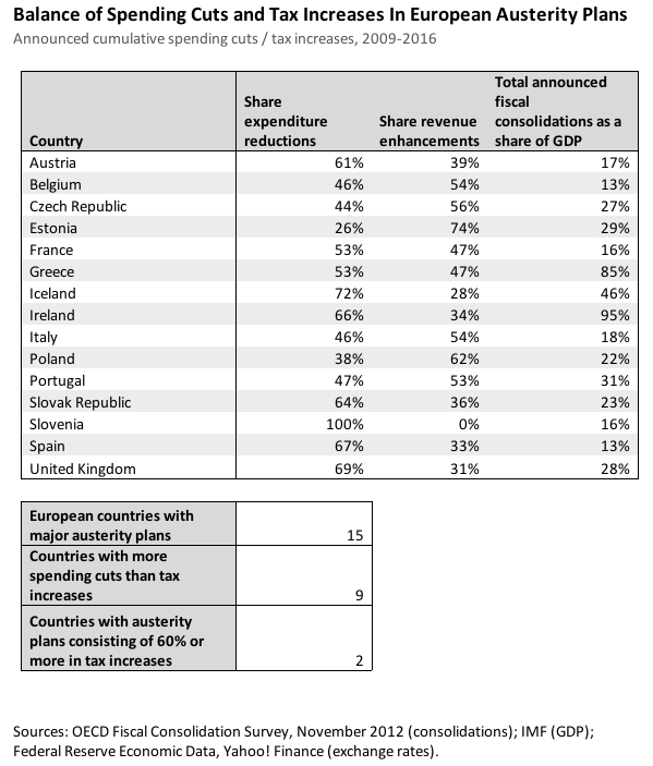
(b) Similarly, you say, in “[the] countries routinely lumped as ‘austere’” spending cuts are “rare.” In its own Restoring Public Finances, 2012 Update, the OECD defines “fiscal consolidations” as “concrete policies aimed at reducing government deficits and debt accumulation, e.g. active policies to improve the fiscal position.” In analyzing the “fiscal consolidations” of each nation, the OECD looked at “expenditure reductions” and “revenue enhancements.” According to the OECD’s own data (please see the attached summary prepared by my staff), of the 15 European nations with major austerity programs, 9 of those countries had more expenditure reductions than revenue enhancements, and only Estonia and Poland’s austerity programs consisted of less than 40% expenditure reductions. How is that rare?

The discrepancy between my data and the Fiscal Consolidation Survey (FCS) data presented in Restoring Public Finances, 2012 Update is that my data is historical and the FCS was a self-reported survey of plans taken in early 2012.[2] The original wording of this question misrepresents the FCS data and puts words in the OECD’s mouth.

Question 1 selectively and deceptively quotes from Restoring Public Finances in the sentence that reads:

In analyzing the “fiscal consolidations” of each nation, the OECD looked at “expenditure reductions” and “revenue enhancements.”

The quoted phrases are severed from context. In Restoring Public Finances, the first use of the words “fiscal consolidation” is in the phrase “fiscal consolidation strategies.”[3] Just below that we have “fiscal consolidation need.” The second paragraph mentions “progress in implementing fiscal consolidation and the further development of the consolidation plans.” Chapter 1 is titled, “Fiscal consolidation targets, plans, and measures in OECD countries.”[4] Each country’s data is presented with a subsection titled “The government’s fiscal consolidation plan.” The plans are reported for dates as late as 2016.

But question 1 refers to “major austerity programs” in the past tense, using the verbs “had” and “consisted of.”

But the original data reflect plans, and span dates in the past and the future. There is no conflict between my claim that spending cuts since 2007 have been rare and the FCS’s claim that spending cuts will become common in the future.

There is overlap between my data and the OECD data behind the Senator’s spreadsheet (2009 in 2 cases, 2010 in 8 cases, and 2011 in 14 cases). But since both sets of data – mine and the Senator’s – were presented in a summarized form, there is no reason the data could not be in harmony for those few overlapping years.

In addition, Question 1 refers to “the OECD’s own data (please see the attached summary prepared by my staff).” But the FCS data is not, as a point of fact, OECD-originated data but data reported by the particular governments of the OECD member states. This is clear in the Foreword to the OECD’s Restoring Public Finances:

The survey is based on self-reporting from governments…. Some countries did not provide data on implemented consolidation (2009/10-11). The Secretariat has included implemented consolidation in 2009-11 based on last year’s report for the most obvious cases. Some countries did not provide cumulative data, so the data have been recalculated into cumulative terms by the Secretariat wherever possible. Some countries did not provide quantified data for the total consolidation period, even if measures were specified.

The OECD has done an excellent job gathering and harmonizing the data gathered in its survey, and OECD staff has been helpful and prompt in responding to requests for documentation.[5] Knut Klepsvik, OECD Senior Policy Analyst, confirmed in personal communication, “The data of the Restoring Public Finances, 2012 Update are based on self-reporting from countries but the OECD Secretariat has performed a data quality control as we do on all surveys. The projections are still the governments’ own estimates and may include more or less optimistic estimates.” The insinuation that the FCS data is superior to data from Statistics OECD[6] is bizarre.

Worse, the summary prepared by your staff[7] and attached to the Questions for the Record is in direct conflict with Figure 1.15 in Restoring Public Finances,[8] which is the OECD’s own calculation of the composition of the reported fiscal austerity plans.

I successfully replicated the data in your staff’s spreadsheet only by making the same error that they did: they treated cumulative data as non-cumulative, vastly overcounting the early years in each country’s record, and grossly exaggerating the total fiscal consolidation in each country. This spreadsheet, while its proportions end up looking similar to the correct ones, is utterly meaningless and I will disregard it.

Turning instead to the OECD’s own summary of the data, in Figure 1.15, the reason that my data do not match is that they are drawn from a different period. The data for 2012 through 2016 are all projections or plans of future changes. The OECD authors recognize the distinction, noting for example, “The OECD has calculated the deviation of the actual fiscal balance in 2010 and 2011 compared to the targeted fiscal balances described in last year’s report.”[9]

By contrast, my data, by design, are dated from before the crisis. Like Figure 1.15, it summarizes several years of data, and finds that spending cuts have been rare. According to OECD data,[10] government consumption grew in 20 of 27 countries from 2007 to 2012 (or 2011 where 2012 data was unavailable). Spending fell in six crisis countries plus the U.K.

As I note in the documentation, government spending as a share of GDP rose in 23 countries. I chose to use the indicator I deemed most accurate, not the one that yielded the most dramatic results.

What is important in determining that spending cuts have been rare is to use a dating convention that captures the full path of fiscal policy over several years. Some will disagree with that dating choice, but it is up to them to prove that their spending cuts do not merely represent the end of temporary spending measures undertaken in the worst years of the crisis.

As I argue in the opening of my testimony, I do not like the term “austerity” because it is overly broad and has meant all sorts of things over the years. Thus, it should be no surprise that I do not favor any single definition of austerity. This debate should persuade observers that the label “austerity” should be dropped in favor of narrower terms like “tax increase” and “entitlement reform.”

For illustrative purposes, I labeled “austere” countries in my two charts. However, each chart does so using a different definition, and the purpose of the charts is more to show how diverse fiscal approaches have been, not to offer a taxonomy of austerity.

As a general rule, I would consider it unlikely that austerity would be an accurate description of a country that had made no policy changes, but perhaps some exception exists.

No.[11] This question is a good reminder of the importance of knowing the context. Had any of the four fast-growing economies in my sample had a revenue rate increase, I would have investigated the narrative to make sure I was not reporting a misleading statistic.

Because Restoring Public Finances is mainly a prospective, not retrospective, publication, its fiscal consolidations are primarily planned, not “undergone.”

In Box 1.1, the OECD’s definition of fiscal consolidation emphasizes the forward-looking nature of this particular report.[12]

In this report, fiscal consolidation is defined as concrete policies aimed at reducing government deficits and debt accumulation…. Merely announcing an ambitious deficit target over the medium term with no accompanying consolidation plan on how to achieve the deficit target is not regarded as consolidation in this analysis. Consolidation plans and detailed measures are given as a per cent of nominal GDP.

The definition provided does not offer a measuring stick for evaluating which countries have undergone major fiscal consolidations.

This is not nit-picking. When the member countries provided data to the OECD, they did so for whatever years they chose, reflecting their different views and plans. That’s why there is 2009 data for only two countries. These data are not designed to look backwards and are sparsely populated for the first two years.

Finding spending cuts in 2010 and 2011 is like finding rapid U.S. GDP growth in 1933 and 1934: out of context, it will give the wrong impression.

Yes, I would absolutely consider it an austerity measure. A major part of my testimony was to argue that one austerity measure – tax increases – was being counteracted by stimulus spending. The tax increase is an austerity measure, as would be mass layoffs. But I am interested in looking at the net effect.

If the social safety net were so generous (or inefficient) that the government spent more on social services for a laid-off worker than it did to employ a worker, then austerity (or its lack) would be the least of the government’s problems.

The early 1990s are a great example of the success of structural reform and spending cuts. Fiscal consolidation from 1993 on featured 67 percent spending cuts and 33 percent tax increases. IMF economists recently quantified a detailed narrative of the tax increases and spending cuts during that era.[13]

Again, cautioning against drawing too much from a single example, the early 1990s featured steady fiscal consolidation in the U.S., as well as welfare reform (a key structural reform) in 1996. The table below shows the fiscal consolidation undertaken each year, and the ensuing real per capita GDP growth.

1990 had fiscal consolidation mainly on the tax side. A recession followed. Consolidation accelerated, with an even tax-spend split over the next two years and the economy recovered, but less rapidly than after most previous recessions.

1993 continued the spending cuts but with few tax increases, and the economy boomed at 2.8 percent growth from 1993 to 1994.

1. Regarding tax increases and spending cuts.
2. How do you define “austerity”? Under your definition, can “austerity” occur in the absence of government action?
3. If, in the absence of government action, the ratio of revenue to GDP increases, would you consider that austerity in the form of a tax increase?
4. Using the OECD’s own definitions of terms [from the OECD’s Restoring Public Finances], do any of nations which have undergone major “fiscal consolidations” lack significant “expenditure reductions.”
5. If the United States laid off 25% of the federal workforce to trim its budget, would you consider that to be an austerity measure? Does your answer depend on how much social-safety-net-program spending increases to support those now-unemployed workers and their families?
6. In your testimony, you stated “higher tax rates slow the economy immediately and depress future growth.” Are you familiar with the U.S. experience in the 1990s, during which tax rate increases in 1993 were followed by 7 years of economic growth at 4% per year, with 23 million new jobs created? How do you explain this prosperity following major tax increases?

The large spending cut and tax increase passed in August 1993 had its greatest effects during 1994.[14] In particular the OBRA-1993 sought major savings from Medicare and federal employee benefits,[15] which are good examples of the structural reforms I recommended in my testimony.

GDP per capita grew only 1.3 percent from 1994 to 1995. That’s not bad, reflecting a private sector that rapidly picked up the slack as government’s growth slowed.

From 1995 to 1998, fiscal consolidation was heavily on the spending side, and growth accelerated to a smoking 3.6 percent and the deficit turned to a surplus.

The fact that growth was strongest right after spending cuts preponderated and weakest when taxes increased most is an excellent exhibit of the case for preferring spending cuts. Using a regression to quantify the correlations,[16] I find that a 0.1 percent of GDP cut in spending is associated with 1.2 percentage point higher GDP growth. And a similar tax increase is associated with 1.4 percentage point lower GDP growth.[17] These coefficients have no applicability out of sample, but they tell us that in the 1990s U.S. higher taxes and lower growth went together like fire and smoke.

Good economists do not draw conclusions based on a handful of data points. The argument against spending cuts leans heavily on blaming Europe’s failed recovery for austerity.  Just as the U.S. experience in the 1990s does not prove that spending cuts are expansionary, the European experience in the 2010s cannot prove that spending cuts are contractionary.

The successful consolidations consisted of 34 percent tax increases.[18] In unsuccessful consolidations (which are about twice as common), tax increases preponderate: 73 percent of the consolidation is on the tax side.

This paper is mainly about political outcomes, showing that you can get reelected even if you cut spending and raise taxes. “Moreover, cabinets that are willing to cut transfers and the government wage bill – traditionally considered the two most politically charged components of spending – are not punished by the voters.”[19]

As such, the paper does not provide a detailed breakdown of taxation and expenditure splits in the fiscal consolidations it considers, nor does it advocate the 34/66 split as ideal. So it’s hard to go beyond reporting the averages, as I did in my testimony.

The final question wants me to endorse non-linear effects of taxation in fiscal consolidation. But there is simply not enough evidence in any of the papers that I cited to argue for a general tipping point in the optimal mix. Nor can I prove it does not exist.

With a dozen years more data to work with, Biggs, Hassett, and Jensen are willing to put an upper bound on the optimal amount of revenue increases: 15 percent,[20] substantially lower than the average successful consolidation in Alesina et al.’s earlier data.

If these numbers seem contradictory, consider a contrived example:

Suppose consolidations that are 5% tax succeed 75% of the time, if they’re 25% tax they succeed 40% of the time, and if they are 100% tax they succeed 20% of the time. After 100 attempts with each policy (5%, 25%, 100%), the average successful policy will be close to 25% tax increases. But the optimal policy will remain 5% tax.

1. Though you warn against combating deficits by raising revenues, you cite a study (Alesina, Perotti, and Tavares, 1998) that found that successful consolidations have included 66% spending cuts. From where did the nations studied generate the other 34% of deficit reduction? Does this study not suggest that revenue has played a critical role in successful deficit-reduction plans?

 

Appendix A: Spreadsheet from Senator Whitehouse’s Questions for the Record.

Appendix B: Documenting the tables in Furth’s Senate Budget Committee Testimony

To inform the arguments made in testimony before the Senate Budget Committee on June 4, 2013, I used data published by the Organisation for Economic Co-operation and Development (OECD). In this note, I will detail my sources, choices, and calculations for the tables I presented.

My goal was to accurately portray the net fiscal effects of policy decisions taken during recent years. As I made very clear in my testimony, I find the word “austerity” too broad for meaningful discussion. I prefer the better defined “fiscal consolidation,” and for policy evaluation, what is really important is distinguishing between tax changes and spending changes. I argue forcefully in favor of structural reform, cautiously in favor of spending cuts, and firmly in opposition to tax increases.

On “austerity” broadly, I have no opinion.

Throughout the testimony, I do not adhere to any particular definition of austerity. Where I labeled countries “austere” in graphs, it was to show that by that metric they were austere. I discuss other metrics that would yield different sets of “austere” countries.

In my testimony, I am careful not to draw any causal conclusions from recent data. I leave the causality to the academic literature, and complement it by documenting what has occurred over the past five years. I also do not discuss Europe’s plans for future policies. Throughout the paper it is abundantly clear that I am discussing what has occurred since 2007, not what may occur next year.

As I will show, the choices I made lead to sober results, and other choices might have led to more exciting but less enlightening graphics.

I first discuss the main choices in the paper. Then I discuss in detail how and why I produced Chart 1 and Table 1. If a reader would like a copy of my data, I would be happy to provide it.

General approach

One of the truisms of academic economics is that “all papers make choices, and this one is no exception.”

I chose to use a data analysis approach, not a narrative approach.[21] Both are valid and valuable. I believe the data analysis approach better lends itself to cross-country comparisons.

Most consequentially, I chose to begin my series prior to the onset of the 2008 financial crisis. This choice reflects the importance of viewing the crisis years as a whole. That is particularly important because many countries engaged in large, temporary deficit spending programs, such as the American Recovery and Reinvestment Act. If one dates from 2009 or 2010, when temporary spending programs peaked, one comes away with the meretricious impression that new policies have cut spending even where policies have not changed but temporary spending has expired and transfer payments have fallen back from their peak.

Almost any data analysis will fail to find extensive austerity, by any definition, over the period from pre-crisis to the present. Likewise, almost any analysis that embarks from the peak of the crisis is likely to find rampant austerity, at least in the Euro Area.

Another approach which I avoid would be to add up all the deficits (adjusted or not) of the past several years. That would be a cheap and easy way to display huge multi-year deficits, but would badly confound policy with relative crisis severity.

Perhaps some wish to make the case that austerity – however they define it – was not a major policy until 2010 or 2011. If so, they have the burden of using the narrative approach or of showing that their results do not mainly stem from policy decisions taken in the 2008-2009 crisis. They also must be careful not to blame economic performance in 2010 on decisions taken in 2011.

Chart 1.

Sources

Chart 1, “Few Governments Have Enacted Real Austerity,” relies on data from the OECD’s Economic Outlook, Volume 2013, Issue 1,[22] which is also referred to as Economic Outlook No. 93. Due to the very timely publication date, I was working from the preliminary version (released May 29, 2013), which is publicly available as an embedded PDF online.[23]

Chart 1 is drawn directly from the table entitled “General government cyclically-adjusted financial balance: surplus (+) or deficit (-) as a percentage of potential GDP.”[24] In order to have the data available in a timely manner, it was manually entered into an Excel spreadsheet and double-checked.

The only calculation in Chart 1 is subtraction to calculate the change in cyclically adjusted financial balance from 2006-2007 to 2012-2013.

Choices

Chart 1 reflects the broad view of fiscal consolidation. Although the measure is imperfect, it is intended to abstract from business-cycle changes in revenues, spending, and GDP. The implication is that it reflects policy, not economic conditions. However, there is always substantial uncertainty about potential GDP in very recent years, so recent (and projected) years are subject to substantial revision.

As mentioned in Footnote 9 of my testimony,[25] I excluded Luxembourg and Norway because their data may not be directly comparable. In Luxembourg’s case, the country’s large proportion of international commuter employees and heavy dependence on the financial sector make it exceptional. Norway’s data excludes off-shore oil revenues, although those are (implicitly) included for other oil producers such as the U.K. and the Netherlands. The exclusions are trivial: both countries would have fallen around the middle of the table in Chart 1.

The only major choice I made in Chart 1 was my choice of beginning and ending years. I chose to average two years together in both cases, because the series is fairly volatile and the economic slowdown before the crisis occurred at different times in different countries. Nor did I want my results to be too heavily influenced by short-lived policies.

I chose to end the series with an average of 2012 and projected 2013 data. Although the OECD publication does not explicitly say so, one suspects that 2012 data, while close to accuracy, are not final numbers. However, the 2012 data were in several cases significantly revised from Economic Outlook No. 92 (December 2012), indicating that new information is being taken into account. As 2013 unfolds and 2012 data is finalized, the results I present may change, but probably not enough to alter the qualitative conclusions.

Likewise, I chose to begin the series with an average of 2006 and 2007 data.

The data in Chart 1 can be read in two ways relative to the question of austerity.

Some reasonable definitions of austerity could rely on the current size of the cyclically adjusted surplus. For instance, one might define countries with a surplus while at least 1 percent below potential GDP as “austere”. Or one might define all countries with a surplus above 2 percent of GDP as austere, regardless of the business cycle.

Alternately, one can define austerity as a change in the underlying cyclically adjusted surplus. This approach implicitly takes politics into account, recognizing that once interest groups have become accustomed to government largesse, they will resist its withdrawal. Thus Greece, while it still has a cyclically adjusted deficit, has narrowed that from 9.6 to 0.7 percent of GDP.

For Chart 1, I chose a definition of austerity as at least a 2 percent tightening of the cyclically adjusted deficit. That takes advantage of a natural discontinuity in the data between Estonia and Italy. But for those who think that a better definition is, for instance, a 1 percent tightening, the data is easily readable and clearly labeled.

Note that the alternate definitions of austerity would give very different results. None of the countries that tightened budgets by at least 2 percent are actually running a structural surplus, by the OECD estimate. This supports my main points: experiences are diverse, austerity is vague, and by any measure it is not as widespread as reported.

Table 1 and Chart 2

Chart 2 is based on data from Table 1. These data are not cyclically adjusted.

Sources

Data for Table 1 come from Statistics OECD[26] and were accessed in the week prior to June 4, 2013. As noted in my testimony, data were not up-to-date for all countries. Switzerland and the non-European countries lacked 2012 data, and I excluded several countries which also lacked 2011 data. This panel is thus more heavily European than Chart 1.

“GDP Growth” is the log difference in GDP between 2012 and 2007, expressed in constant 2005 USD, current PPP (purchasing power parity). I record the log difference as a percentage change for expositional ease, as noted in a footnote. One factor I did not account for in this or other series is the growth of population.

“Government Consumption Growth” is derived from the OECD series “GP3P: Final Consumption Expenditure.”[27] I convert it to constant 2005 USD using PPP exchange rates and the U.S. consumer price index, and take the log difference from 2007 to 2012 (or 2011).

“Transfers” is similarly derived from the sum of OECD series “GD62_631XXP: Social benefits + Social transfers in kind (via market producers), payable” and “GD7P: Other current transfers, payable.”[28]

“Change in Revenue Rate (share of GDP)” is derived from “GTR: Total General government revenue.”[29] The figures listed are the percent of GDP difference.

“Actual 2012 Surplus or Deficit (% of GDP)” is derived from “GB9: Net lending (+)/Net borrowing (-),”[30] and reported as the 2012 (or 2011) ratio of net lending to GDP. Because the OECD reports general government statistics, it would not have been accurate, for instance, to use the (available) 2012 U.S. federal deficit in place of series GB9.

Choices

The most difficult choices in this exposition relate to presenting the growth of components of government income and spending. I chose the methods I best judged would give accurate comparisons across the various phases of the business cycle in which OECD countries presently find themselves.

I took my cue from the ways in which government spending and revenues are generally decided. Consumption is usually statutory, and – absent policy change – does not change drastically with the business cycle. Tax policy is a set of progressive rates, not lump sums, and as a consequence the revenue rate is procyclical. Transfers are composed of strongly procyclical income support and old-age pensions, which ought to be acyclical.

The current archetype of austerity is a country that has cut spending and raised taxes at the same time. Relevant to the present debate is just how much of each is taking place.

One expects consumption to fall, on net, in austere countries. After all, most forms of government consumption have spending levels set by statute, and some government consumption is specifically tied to a revenue stream, leading to mild pro-cyclicality (such as in American municipalities).

Another reasonable way to present these data would be to look at countries where government spending has fallen as a share of GDP. That yields similar results, but they are less illuminating: only the Czech Republic, Ireland, Israel, and Portugal saw a drop.

Thus, a definition based on government consumption as a share of GDP rather than the level of government consumption would find even less austerity than the measure I chose.

It was not obvious to me which was best to present changes in government transfer payments. A draft version of Table 1 presented both “Transfers Growth” and “Transfer Rate Change (% of GDP).” The results were very similar: only fast-growing Israel had transfers fall as a share of GDP.

Some have protested that high transfer growth reflects weakening economies. If that is the case, the data would show that the strongest economies had less transfer growth. There’s a correlation between transfer growth and GDP growth, but it’s in the wrong direction (0.5) and depends heavily on the Greece data point. Stipulating that the zero growth of transfers in Greece and Hungary strongly suggests statutory transfer cuts, there’s little evidence of austerity in the sector beyond Greece, Hungary, and maybe Italy and Sweden. And even in those cases, the “cuts” still leave transfers growing as a share of GDP.

Presenting taxation as a revenue rate was the easiest choice. Revenue collection is roughly proportional to GDP and progressive in income. If one looked only at total revenue collected, one would find that growing economies increased revenues and shrinking economies lost revenue (proportionality). That sheds no light on austerity.

Instead, controlling for proportionality, I used the fact that progressivity generally pushes the revenue rate down in a slow economy. Thus, where I observed the revenue rate rising substantially in depressed economies, it would be strong evidence that tax rates have risen.

The change in the revenue rate is mixed, and the median change is just below zero. While that is what one might expect during an era of average growth, the many countries that raised revenue rates despite a shrinking overall economy are the strongest evidence of “austere” policies that I found in the data.

Philosophically, using revenue rates as an indicator of tax rates reflects my neo-classical economic beliefs. I believe that tax rates are the locus of the distorting, welfare, and growth effects of taxation. A Keynesian might be more inclined to focus on tax revenues.

The final column of Table 1 was included for reference, and is not mentioned in the text of my testimony.

---

The Heritage Foundation is a public policy, research, and educational organization recognized as exempt under section 501(c)(3) of the Internal Revenue Code. It is privately supported and receives no funds from any government at any level, nor does it perform any government or other contract work.

The Heritage Foundation is the most broadly supported think tank in the United States. During 2013, it had nearly 600,000 individual, foundation, and corporate supporters representing every state in the U.S. Its 2013 income came from the following sources:

Individuals 80%

Foundations 17%

Corporations 3%

The top five corporate givers provided The Heritage Foundation with 2% of its 2013 income. The Heritage Foundation’s books are audited annually by the national accounting firm of McGladrey, LLP.

Members of The Heritage Foundation staff testify as individuals discussing their own independent research. The views expressed are their own and do not reflect an institutional position for The Heritage Foundation or its board of trustees.

 

Endnotes

[1] “The standard rate of VAT increased from 17.5 per cent to 20 per cent on 4 January 2011.” Source: GOV.uk, “VAT rates,” https://www.gov.uk/vat-rates (accessed June 6, 2013).

[2] Organisation for Economic Co-operation and Development, Restoring Public Finances: 2012 Update, p. 72.

[3] Ibid., p. 3.

[4] Ibid, p. 17.

[5] For example, Knut Klepsvik, OECD Senior Policy Analyst, clarified the sources of Estonia’s data in personal communication: “Concerning Estonia, we enquired if their figures were cumulative or incremental. The Estonia authorities confirmed that all the expenditure measures are cumulative but there are some one-off revenue measures that aren’t cumulative. However, Estonia don't have a consolidation plan after 2010 (Box 1.6) but have implemented large front-loaded consolidation since 2008. We have interpreted their response as Estonia is withdrawing from fiscal consolidation and gradually are removing expenditure measures which may be considered as stimulating the economy.” Reproduced as received.

[6] Statistics OECD, http://stats.oecd.org/.

[7] I have included the summary as Appendix A.

[8] OECD, Restoring Public Finances: 2012 Update, p. 41. Data are downloadable in Excel format from http://dx.doi.org/10.1787/888932696894.

[9] OECD, Restoring Public Finances: 2012 Update, p. 27. Emphasis added.

[10] See Appendix B for the titles of the particular series I used and the calculations I performed.

[11] Given the recent “fiscal cliff,” it is worth stipulating that policy expiration is a form of government action.

[12] OECD, Restoring Public Finances: 2012 Update, p. 18.

[13] Pete Devries, Jaime Guajardo, Daniel Leigh, and Andrea Pescatori, “A New Action-based Dataset of Fiscal Consolidation,” IMF Working Paper 11/128, June 2011, pp. 81-85.

[14] Devries, Guajardo, Leigh, and Pescatori, “A New Action-based Dataset of Fiscal Consolidation,” p. 84.

[15] Congressional Budget Office, “The Economic and Budget Outlook: An Update,” September 1993, p. 29, http://cbo.gov/sites/default/files/cbofiles/ftpdocs/76xx/doc7670/09-1993-outlookentirerpt.pdf.

[16] I am not claiming causation on the basis of these nine data points. I include a time trend.

[17] Both coefficients are statistically significant at the 95 percent level, but it’s still only a correlation.

[18] Alberto Alesina, Roberto Perotti, José Tavares, “The Political Economy of Fiscal Adjustments,” in Brookings Papers on Economic Activity, Vol. 1998(1), Maurice Obstfeld and Barry Eichengreen eds., 1998, p. 201.

[19] Alesina, Perotti, and Tavares, “The Political Economy of Fiscal Adjustments,” p. 198.

[20] Andrew G. Biggs, Kevin A. Hassett, and Matthew Jensen, “A Guide for Deficit Reduction in the United States Based on Historical Consolidations That Worked,” American Enterprise Institute Economic Policy Working Paper 2010-04, December 2010, p. 13.

[21] A narrative approach involves cataloging, categorizing, and quantifying historical events – policy changes, in this case. Thus a narrative approach would record (for instance) each tax cut and tax increase, its rate changes, its expected or realized revenue gains, and the justification given by its enactors.

[22] OECD iLibrary, OECD Economic Outlook, Volume 2013, Issue 1, May 29, 2013, http://www.oecd-ilibrary.org/economics/oecd-economic-outlook-volume-2013-issue-1_eco_outlook-v2013-1-en (accessed June 5, 2013).

[23] OECD Publishing, OECD Economic Outlook, Volume 2013, Issue 1, http://www.keepeek.com/Digital-Asset-Management/oecd/economics/oecd-economic-outlook-volume-2013-issue-1_eco_outlook-v2013-1-en (accessed June 5, 2013).

[24] OECD Publishing, OECD Economic Outlook, Volume 2013, Issue 1, p. 238. The previous edition of Economic Outlook labeled this data “Statistical Annex Table 28” and used the word “balances” instead of the phrase “financial balances.”

[25] Salim Furth, “Testimony on the Fiscal and Economic Effects of Austerity before the Committee on the Budget,” June 4, 2013, p. 4.

[26] Statistics OECD, http://stats.oecd.org/.

[27] Statistics OECD, 12. Government deficit/surplus, revenue, expenditure and main aggregates, http://stats.oecd.org/Index.aspx?DatasetCode=SNA_TABLE12 (downloaded May 29, 2013).

[28] Ibid.

[29] Ibid.

[30] Ibid.