My name is David Kreutzer. I am Research Fellow in Energy Economics and Climate Change at The Heritage Foundation. The views I express in this testimony are my own, and should not be construed as representing any official position of The Heritage Foundation.
Carbon Taxes, Energy Costs, and Economic Activity
Hydrocarbon fuels provide 85 percent of energy in the U.S. So, a tax on carbon-dioxide will drive up energy costs. These higher energy costs work their way through the economy raising costs of production, reducing income and reducing employment. Analyses by both The Heritage Foundation and the Energy Information Administration project impacts of carbon taxes that show employment losses exceeding 1,000,000 jobs and income losses (GDP) exceeding a trillion dollars by 2030.
Taxes have two general categories of costs. The first is the tax revenue, called the direct burden in economic jargon. The second is the cost imposed by the tax’s price distortions, called the excess burden in economic jargon. A simple (if extreme) example will illustrate these different impacts.
Suppose there is a $3,000,000 per gallon tax imposed on dairy products and with this tax in place a single gallon of ice cream is purchased each year. The tax revenue (direct burden) is $3,000,000. The excess burden is the value lost by destroying the dairy industry—farmers, processors, vendors, etc.—minus any gains by those who produce and sell whatever substitutes replace a portion of the lost dairy products. In addition the excess burden would include the lost value to consumers who give up ice cream, milk, cheese, etc. for less appealing alternatives.
The economic impacts outline above (and discussed further below) include only the excess burden. At least in the Heritage analysis, the tax revenue is rebated immediately and directly to taxpayers. What remains is the damage done to the economy.
Boxer-Sanders Carbon Tax
In 2013 Senators Barbara Boxer (D-CA) and Bernie Sanders (I-VT) proposed a carbon tax in their Climate Security Act of 2013.[1] The tax started at $20 per metric ton and would rise by 5.6 percent per year, reaching $50 per metric ton by 2030 (the endpoint for the Heritage analysis).
Using the Heritage Energy Model (HEM), a derivative of the Energy Information Administration’s National Energy Modeling System (NEMS), Heritage projected what the economic impacts would have been had the bill become law.[2]
The impacts would have included (dollar values are adjusted for inflation):
- GDP loss of $146 billion in 2030
- A family of four losing more than $1,000 of income per year,
- Over 400,000 lost jobs by 2016,
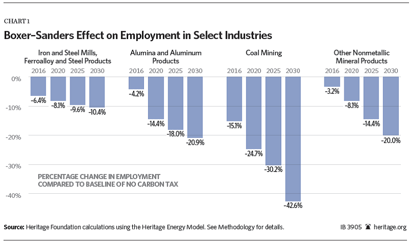
- Coal production dropping by 60 percent and coal employment dropping by more than 40 percent by 2030,
- Gasoline prices rising $0.20 by 2016 and $0.30 before 2030, and
- Electricity prices rising 20 percent by 2017 and more than 30 percent by 2030.
Though renewable energy grew compared to baseline levels, it wasn’t enough to make up for the lost hydrocarbon energy. In addition it is certain that businesses and households economized on energy use both by doing without and by employing more energy efficient technologies. These responses would stimulate employment in certain sectors, but the net effect is an overall loss in employment. The projected employment loss for 2016 was 400,000 jobs. Of course the energy-dependent sectors would suffer relatively larger job losses. Chart 1 from the Heritage analysis shows job losses as a percent of baseline employment.
In early 2013, a Heritage paper looked at the economic impacts of a carbon tax that was included as a side case in the EIA’s Annual Energy Outlook 2012.[3] That analysis noted the following impacts of a $25 per ton tax on carbon dioxide:
- Cut the income of a family of four by $1,900 per year in 2016 and lead to average losses of $1,400 per year through 2035;
- Raise the family-of-four energy bill by more than $500 per year (not counting the cost of gasoline);
- Cause gasoline prices to increase by up to $0.50 gallon, or by 10 percent on an average gallon price; and
- Lead to an aggregate loss of more than 1 million jobs by 2016 alone.
Again, it should be noted that the NEMS and the HEM both include the changes in behavior and investment in energy-saving technology that firms and households will undertake to adjust to higher prices. So, the projected income and job losses are over and above any offsetting gains found in industries and services that provide low-carbon and no-carbon alternatives.
The Annual Energy Outlook 2014 (the most current edition) also has a $25 per ton carbon-tax side case.[4] Again the GDP losses are significant, exceeding $150 billion for many years, and the jobs losses are severe, with employment in some years falling below the no-carbon-tax reference case by more than one million jobs.
So, carbon taxes will drive up energy costs, reduce employment, and cut income.
Impact on Climate
Some would argue that the CO2 reductions create benefits from reduced global warming and the value of these benefits more than offsets the cost of a million lost jobs and trillions of dollars of lost income. There are several ways of looking at these suggested benefits.
Estimates of a carbon tax’s impact on world temperature do not lend much support for a carbon tax. Climatologists Pat Michaels and Chip Knappenberger provides an online calculator to estimate the impact of various cuts in CO2 emissions.[5] The calculations are based on the MAGICC model developed at the National Center for Atmospheric Research.
The AEO2014 side case for the $25 per ton carbon tax would cut energy-related CO2 emissions by about 50 percent by 2050 (overall emissions would probably drop by a slightly smaller percentage). These cuts translate to a temperature moderation of about 0.05 degrees centigrade (about 0.09 degrees Fahrenheit) by the end of this century. Few would argue that this virtually unmeasurable impact is worth the million lost jobs and trillions of dollars of lost income.
Even eliminating carbon dioxide emissions entirely and assuming the highest sensitivity of world temperature to carbon dioxide levels (which happens to be the sensitivity that is furthest from that in recent research) would project a temperature moderation of less than 0.2 degree centigrade.[6] Of course, eliminating CO2 emissions entirely, if possible, would have much higher costs than even those of the $25 carbon tax modeled by the EIA or the Boxer-Sanders tax modeled by Heritage.
The Social Cost of Carbon
The social cost of carbon (SCC) is, in theory, a measure of the damage done to future economies from the emission of another ton of CO2 for the year in which the CO2 is emitted. In concept, the CO2 emitted adds a warming effect to the atmosphere for the year in which it was emitted as well as subsequent years (to varying degrees) for centuries to come. The added warming in each year will have economic impacts from the warming and from sea-level rise. The present value of these damages is summed to get the social cost of carbon for the year of emission.
An interagency working group (IWG) produced a technical support document (TSD) in 2013 setting out a schedule of SCC values by year and by the discount rate used in the present-value calculations. The IWG used three integrated assessment models (IAMs) to estimate the SCC values for each year. Though interesting theoretical exercises, the information needed to flesh out the IAMs does not exist. As a result the arbitrary values are inserted to paper over the missing critical information generating useless output from technically sophisticated models. Others have noted these fatal problems with the IAMs.[7]
In addition, the IWG ignored guidance from OMB regarding appropriate discount rates and did not use the most up to date equilibrium climate sensitivity distributions.
Heritage analyzed two of the three models used by the IWG—the DICE model and the FUND model. The proprietor of the third model, PAGE, insists on the right of co-authorship for any publication using his model. Because this insistence seriously compromises the independence of evaluating the model, Heritage did not do so. This also raises a question as to the propriety of basing costly federal regulation, at least in part, on a model that cannot be rigorously and independently evaluated.
When Heritage evaluated the FUND and DICE models it was clear that the resulting SCC estimates were very sensitive to the choice of discount rates and equilibrium climate sensitivity.
Equilibrium Climate Sensitivity
Although global-warming activists consistently claim that the science on global warming is settled, anyone who has any familiarity with the scientific process would understand that research is a constant, ongoing process. For instance, one critical component of unsettled science is how much warming will be generated by a given increase in atmospheric CO2 levels. This important (possibly all-important) relationship is called the ECS. The ECS typically gives an expected warming in degrees centigrade for a doubling of atmospheric CO2 levels.
Instead of using a single number, or point estimate, for the ECS, the IAMs use a distribution of possible values for the ECS. In essence, the distribution is a spectrum of values in which potential temperatures are weighted by their probability of occurrence. Because of the myriad factors that affect measured temperatures, estimates of ECS distributions are themselves uncertain and evolve as new data and theory are added to the process.
The IAMs used by the IWG to estimate the SCC are grounded on the specification of such an ECS distribution. Since 2010, the IWG has used an ECS distribution based on an academic paper by Gerard Roe and Marcia Baker published seven years ago.[8] Since then, a number of updated ECS distributions have been estimated, suggesting lower probabilities of extreme global warming.[9]
For instance, substituting the ECS of Otto et al. for the outdated Roe and Baker distribution, used in the 2013 TSD, causes the SCC for 2020 to drop 41 percent with the DICE model and over 60 percent with the FUND model.[10] There were similar reductions on the SCC for other years as well.
Discount Rate
Swapping income today for greater income in the future is investment. The logic underpinning a carbon tax is the same. Lower GDP today will provide even greater benefits in the future. Because there are many investment opportunities that can swap current income for even greater future benefits it is necessary to compare alternative investments to investments in moderating global warming. In the jargon of Econ 101, “what is the opportunity cost” of such an investment—what is the alternative investment of the same magnitude that would provide the greatest alternative future benefit?
Stated another way, the tradeoff is this: Instead of forcing the current generation to invest in climate policy, they could be forced to invest in infrastructure, machinery, tools, factories or anything else that would lead to greater production (and therefore consumption) capacity in the future. It would not make sense to invest for future generations at three percent when, instead, they could reap the reward of a seven percent return.
Discounting is the tool used to make the comparisons and the correct rate is critical. Office of Management and Budget guidance stipulates that cost-benefit analysis should use discount rates of three and seven percent. [11]
The IWG’s TSD used 2.5 percent, 3 percent, and 5 percent discount rates but neglected to report SCC values based on 7 percent. The IWG settled on three percent as the most reasonable discount rate and those are the values that have been used in regulatory rule-making. Comparing the SCC values in the DICE model for the year 2020, Heritage found the value dropped nearly 85 percent when the 7 percent discount rate was used. In the FUND model the SCC drops more than 100 percent and actually goes negative when the 7 percent discount rate is used.
Following the logic of a carbon tax implies that CO2 emissions should be subsidized when the SCC is negative.
Declining Discount Rates and Economic Growth Rates
The case for very low discount rates (declining discount rates) is derived from Martin Weitzman’s 1998 article on discounting the far-distant future [12]. Weitzman argues that when there is uncertainty about future discount rates, the lowest discount rate is the appropriate rate for “the far-distant future.” In practice this has led to the case for using declining discount rates (DDRs). That is, the farther in the future a cost is incurred or a benefit is received the lower should be the discount rate.
A recent article in Science, Arrow et al., provides a summary of and supporting example for the declining discount rate argument.[13] However a close reading of both the Science article and Wietzman’s original article reveals just how critical, and arguably contrived, are the assumptions needed to justify declining discount rates. Nevertheless, even with the assumptions ceded, declining discount rates cannot be used with the IAMs as set up in the IWG’s analysis. The low discount rates that motivate DDRs require extended periods of stagnant growth; and the growth rates used by the IWG in the IAMs are too high to meet this criterion.
The following table is taken from Arrow, et al.:
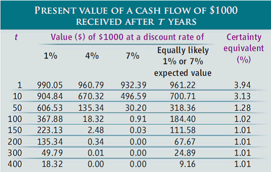
The column heading “Equally likely 1% or 7% expected value” and their description in the text, “Suppose that we think the interest rate is equally likely to be 1% or 7% in 100 years,” could reasonable be interpreted as implying an annual coin flip to choose the discount rate. Instead, they have averaged the present value of two very unlikely outcomes—the first where the chosen interest rate is 1 percent every year for 100 years and the other is where the chosen interest rate is 7 percent every year for 100 years. Though the discussion about correlated discount rates later in the paper alludes to this assumption, many, if not most, readers are likely to believe the odds of 1 or 7 are equally likely in every year. Under the assumption that one and seven have an equal chance every year, the two cases shown above each have a 7.9 x 10⁻³¹ chance of occurring. Most of the paths in the example above will have combinations of some years with a one-percent rate and other years with a seven-percent rate.
Extreme Assumptions Needed for Declining Discount Rates
The Science paper refers to several other papers that also derive these declining discount rates. A necessity for all of them is that the lower discount rate must be in force for an extended period.
For a 300-year time horizon, the simplest split of equally likely one-percent and seven-percent discount rates would be 150 years at 1 percent and 150 years at 7 percent. Discounting $1,000 for 150 years at one percent gives a present value of $224.79. Discounting this value for the remaining 150 years (for a total of 300 years) at 7 percent gives an ultimate present value of $0.0088. Note that using the average discount rate of 4 percent for the whole 300 years gives a present value of $0.0078. In fact, for the present value to even reach as high as $1.00, the one percent discount rate has to apply to at least 232 of the 300 years. If one and seven are equally likely for each of those years, the probability of this occurring is 2.05 x 10⁻²².
Correlated Discount Rates and Economic Growth Rates
To extricate themselves from the dismal probabilities of the previous paragraph, proponents of declining discount rates appeal to the possibility of correlated discount rates. In essence, the coin flips stop early in the game and we are stuck with the rate chosen on that last flip, which at the time of analysis is unknown.
Weitzman illustrates the uncertainty this way:
“When I try to imagine how the future world might look a century from now, I start by trying to conceptualize how people a century ago might have attempted to envision our world today. We have available now some important technologies, like computers or airplanes, that were essentially unimaginable 100 years ago. Maybe a now unimaginable ‘photon-based technology’ will replace today’s electronic technology and deliver such prodigious rates of technological progress with a clean environment that historians then will look back on the previous 100 years and smile at the modest projections of even the growth optimists at the close of the twentieth century. Or, who knows, maybe a century from now people will feel crowded and polluted and very disappointed in a pace of technological change that failed to maintain the productivity growth of the ‘golden age’ of the industrial revolution during the earlier two centuries from 1800 to 2000.”
The people in the future envisioned by the IWG (and embedded in their IAMs) need not worry. They will not be disappointed because the IWG assumes future growth in per capita GDP that actually exceeds that of the U.S. for the past two centuries.
The per capita GDP growth rates for the reference scenarios listed by the IWG ranged from 1.58 percent to 2.03 percent per year with an average of 1.8 percent per year. On the other hand the Maddison Project estimates per capita GDP levels for the U.S. that grew only 1.56 percent per year from 1800 to 2000.[14] Over those same two centuries the real compounded annual rate of return in U.S. stock markets has been a “remarkably stable” 6.8 percent per year.[15] It would be reasonable to assign an even higher projected rate of return on capital in an environment where growth is projected to be in excess of 1.56 percent.
In short, the growth rates built into the IAMs exceed that of the past two centuries in the U.S. (and the world) and therefore rule out the possibility that Weitzman offers as justification for the very low discount rates. The IWG cannot simultaneously entertain arguments for low discount rates and project high GDP growth rates. At least until economic growth in the IAMs is re-worked to match the lower rates implied by DDRs there can be no argument for DDRs in the IAMs.
Summary
- Carbon taxes are bad for the economy as economic analysis by both the Heritage Foundation and the U.S. Energy Information Administration have projected.
- Reducing CO2 with a carbon tax will have at most tenths of a degree moderation in global warming.
- Social cost of carbon estimates from the Interagency Working Group’s 2013 technical support document are simply not credible and cannot justify the million lost jobs and trillions of dollars lost income from a carbon tax.
Appendix
Overview of Heritage Energy Model.
The Heritage Energy Model (HEM) is a derivative of the National Energy Model System (NEMS). [16] NEMS is used by the Energy Information Administration (EIA) of the Department of Energy as well as various nongovernmental organizations for a variety of purposes, including forecasting the effects of energy policy changes on a plethora of leading economic indicators. The methodologies, assumptions, conclusions, and opinions in this report are entirely the work of statisticians and economists at The Heritage Foundation’s Center for Data Analysis (CDA) and have not been endorsed by and do not necessarily reflect the views of the developers of NEMS.
HEM is based on well-established economic theory as well as historical data and contains a variety of modules that interact with each other for long-term forecasting. In particular, HEM focuses on the interactions among (1) the supply, conversion, and demand of energy in its various forms; (2) American energy and the overall American economy; (3) the American energy market and the world petroleum market; and (4) current production and consumption decisions as well as expectations about the future[17] These modules include:
- a Macroeconomic Activity Module,[18]
- a Transportation Demand Module,
- a Residential Demand Module,
- an Industrial Demand Module,
- a Commercial Demand Module,
- a Coal Market Module,
- an Electricity Market Module,
- a Petroleum Market Module,
- an Oil and Gas Supply Module,
- a Renewable Fuels Module,
- an International Energy Activity Module, and
- a Natural Gas Transmission and Distribution Module.
HEM is identical to the EIA’s NEMS with the exception of the Commercial Demand Module. Unlike NEMS, this module does not make projections regarding commercial floor-space data of pertinent commercial buildings. Other than that, however, HEM is identical to NEMS.
Overarching the above modules is an Integrating Module that consistently cycles, iteratively executing and allowing the various modules to interact with each other. Unknown variables that are related (such as if they are a component of a particular module) are grouped together, and a pertinent subsystem of equations and inequalities corresponding to each group is solved via a variety of commonly used numerical analytic techniques, using approximate values for the other unknowns. Once these group’s values are computed, the next group is solved similarly and the process iterates. Convergence checks are performed for each price and quantity statistic to determine whether subsequent changes in that particular statistic fall within a given tolerance. After all group values for the current cycle are determined, the next cycle begins. For example, at cycle j, a variety of n pertinent statistics represented by the vectoris obtained.[19] HEM provides a number of diagnostic measures, based on differences between cycles, to indicate whether a stable solution has been achieved.
Carbon Tax Simulations and Diagnostics.
We used the HEM to analyze the economic effects of instituting the Boxer–Sanders proposal. HEM is appropriate for this analysis, as similar models have been used in the past to understand the economic effects of other carbon tax proposals.[20] In particular, we conducted simulations running a carbon fee that started in 2014 at $20 (in 2013 dollars) and increased by 5.6 percent per year and compared this against a baseline model without any carbon tax. We chose a revenue-neutral carbon tax where 100 percent of the carbon tax revenues are returned directly to taxpayers. We ran the HEM for 12 cycles to get consistent feedback into the Macroeconomic Activity Module, which provided us with the figures presented in this study.
The diagnostic tests, based on differences between cycles, at the end of the 12 runs suggested that the forecasts provided by the model had stabilized. The 12 cycles were therefore sufficient to attain meaningful convergence, thus providing us with macroeconomic statistics from which we can make informative inferences.
Endnotes
[1] Climate Protection Act of 2013, http://www.sanders.senate.gov/imo/media/doc/0121413-ClimateProtectionAct.pdf (accessed September 10, 2014).
[2] Kreutzer, David W. and Kevin Dayaratna, “Boxer–Sanders Carbon Tax: Economic Impact,” Heritage Foundation Issue Brief #3905, April 11, 2013, http://www.heritage.org/research/reports/2013/04/boxer-sanders-carbon-tax-economic-impact (accessed September 10, 2014).
[3] Kreutzer, David W. and Nicolas Loris, “Carbon Tax Would Raise Unemployment, Not Swap Revenue,” Heritage Foundation Issue Brief #3819, January 8, 2013, http://www.heritage.org/research/reports/2013/01/carbon-tax-would-raise-unemployment-not-revenue
[4] U.S. Energy Information Administration, Annual Energy Outlook 2014 Table Browser, “Reference” and “Greenhouse gas $25” cases, Macroeconomic Indicators, http://www.eia.gov/oiaf/aeo/tablebrowser/#release=AEO2014&subject=5-AEO2014&table=18-AEO2014®ion=0-0&cases=co2fee25-d011614a,ref2014-d102413a (accessed September 11, 2014).
[5] Michaels, Patrick J. and Paul C. “Chip” Knappenberger, “Current Wisdom: We Calculate, You Decide: A Handy-Dandy Carbon Tax Temperature-Savings Calculator, Cato Institute, July 23, 2013, http://www.cato.org/blog/current-wisdom-we-calculate-you-decide-handy-dandy-carbon-tax-temperature-savings-calculator (accessed September 11, 2014).
[6] For examples of recent estimates of climate sensitivity see Nicholas Lewis, “An Objective Bayesian Improved Approach for Applying Optimal Fingerprint Techniques to Estimate Climate Sensitivity,” Journal of Climate, Vol. 26, No. 19 (October 2013), pp. 7414–7429; Alexander Otto et al., “Energy Budget Constraints on Climate Response,” Nature Geoscience, Vol. 6, No. 6 (June 2013), pp. 415–416; Magne Aldrin et al., “Bayesian Estimation of Climate Sensitivity Based on a Simple Climate Model Fitted to Observations of Hemispheric Temperatures and Global Ocean Heat Content,” Environmetrics, Vol. 23, No. 3 (May 2012), pp. 253–271.
[7] For instance, Robert Pindyck says that “IAM-based analyses of climate policy create a perception of knowledge and precision, but that perception is illusory and misleading.” Robert Pindyck, “Climate Change Policy: What Do the Models Tell Us?” Journal of Economic Literature, September 2013, pp. 860–872. Also see Anne Smith et al., “A Review of the Damage Functions Used in Estimating the Social Cost of Carbon,” American Petroleum Institute, February 20, 2014, http://www.afpm.org/WorkArea/DownloadAsset.aspx?id=4111 (accessed September 11, 2014).
[8] Gerard H. Roe and Marcia B. Baker, “Why Is Climate Sensitivity So Unpredictable?” Science, Vol. 318, No. 5850 (October 26, 2007), pp. 629–632.
[9] See supra note 6.
[10] Using the 3 percent discount rate chosen by the IWG.
[11] U.S. Office of Management and Budget, “Regulatory Analysis,” Circular A-4, September 17, 2003, http://www.whitehouse.gov/omb/circulars_a004_a-4/ (accessed September 11, 2014).
[12] Weitzman, Martin L., “Why the Far-Distant Future Should Be Discounted at Its Lowest Possible Rate,” Journal of Environmental Economics and Management, Vol. 36, pp. 201-208, 1998.
[13] Arrow, K, et al., “Determining Benefits and Costs for Future Generations,” Science, July 26, 2013, Vol. 341, pp 49-50.
[14] Bolt, J. and J. L. van Zanden (2013). The First Update of the Maddison Project; Re-Estimating Growth Before 1820. Maddison Project Working Paper 4, http://www.ggdc.net/maddison/maddison-project/home.htm (accessed February 26, 2014).
[15] Siegel, Jeremy J., The Concise Encyclopedia of Economics: Stock Market, 2nd ed., Library of Economics and Liberty, http://www.econlib.org/library/Enc/StockMarket.html (accessed February 26, 2014).
[16] U.S. Department of Energy, Energy Information Administration, “The National Energy Modeling System: An Overview,” http://www.eia.gov/oiaf/aeo/overview/pdf/0581(2009).pdf (accessed April 3, 2013).
[17] Ibid., pp. 3–4
[18] HEM’s Macroeconomic Activity Module makes use of the IHS Global Insight model, which is used by government agencies and Fortune 500 organizations to forecast the manifestations of economic events and policy changes on notable economic indicators. As with NEMS, the methodologies, assumptions, conclusions, and opinions in this report are entirely the work of CDA statisticians and economists and have not been endorsed by and do not necessarily reflect the view of the owners of the IHS Global Insight model.
[19] S. A. Gabriel, A. S. Kydes, and P. Whitman, “The National Energy Modeling System: A Large-Scale Energy-Economic Equilibrium Model,” Operations Research, No. 49 (2001), pp. 14–25.
[20] The Department of Energy, for example, has used NEMS to evaluate some carbon tax proposals. See, for example, U.S. Department of Energy, Energy Information Administration, “AEO Table Browser,” http://www.eia.gov/oiaf/aeo/tablebrowser/ (accessed April 2, 2013).