Unions do not provide general economic benefits to non-union workers that could justify forcing non-union workers to pay union dues. The National Labor Relations Act provides that a majority of workers in a bargaining unit of a company may elect to have a union represent all the unit’s workers, whether they are members of the union or not, in negotiations with company management. In half the states, the union can extract compulsory union dues from all workers in the unit, even if they are not union members. In the other half of the states, known as right-to-work (RTW) states, the non-union workers have the freedom individually to decide for themselves whether or not the labor union deserves their financial support. Evidence shows that unions do not provide general economic benefits that would justify forcing workers who are not members of a union to pay union dues.

A deeper look at the evidence shows that unions do not increase wages overall. Unions function as labor monopolies: They raise wages for their members by reducing employment opportunities for non-union workers. As the U.S. economy has become more competitive, unions have lost most of their power to do this. Recent studies have found that workers who vote to unionize earn no more than workers who remain non-union. Union dues do not purchase higher wages.

Right-to-work laws present an interesting economic test of whether unions raise average wages. Unions have considerably fewer members in RTW states. If these states have lower wages, it could suggest that unions increase overall living standards. However, if their real wages are no different, it strongly suggests they do not.

Recently, the union-backed Economic Policy Institute (EPI) published a report arguing that RTW laws do, in fact, reduce wages. They argue that otherwise comparable workers have 3 percent lower real wages in states with voluntary dues.

The Heritage Foundation’s Center for Data Analysis (CDA) replicated this study and found that EPI only partially controlled for cost-of-living differences among states. Using EPI’s preferred model, but fully controlling for cost-of-living differences, shows that private-sector workers have the same purchasing power in RTW as in non-RTW states. Right-to-work laws do appear to slightly reduce the pay of government employees, possibly by reducing their ability to elect sympathetic politicians. Further, workers in RTW states have one percentage point lower unemployment rates. Unions do not provide broad-based economic benefits that justify forcing workers to purchase their services.

Unions and Wages

The EPI is a union-backed think tank with a board of directors chaired by AFL-CIO President Richard Trumka.[1] Nine other senior union officials sit on EPI’s board.[2]

EPI studies argue that the decline of union membership since the 1970s has depressed wages and that RTW laws lower workers’ pay.[3] The EPI has argued strongly that union members earn more than non-union workers and that, if unions can raise wages for their members, expanding union representation would give many workers a raise.[4] On this theory—that the actions of unions deliver economic benefits to non-union workers that justify compelling non-union workers to pay dues to the union—some politicians have voted to take away the freedom of non-union workers to decide individually for themselves whether or not the labor union deserves their financial support.

A deeper look at the evidence shows that unions do not promote general prosperity that justifies compelling non-members to pay dues to unions.

Unions as Labor Monopolies

The argument that unions raise average wages runs contrary to economic theory. In economic terms, unions function as labor monopolies or cartels: They try to control the supply of labor in an industry in order to drive up its price—wages. As with any monopoly, the benefits to union members come at the cost of greater losses to the rest of society.[5]

The United Auto Workers (UAW) union illustrates this dynamic. In the 1930s and 1940s, the UAW organized the entire U.S. auto industry. The union used its monopoly to impose expensive compensation packages on the Detroit automakers. Until the 2008 financial crisis, UAW members received more than $70 an hour in wages and benefits.[6]

The UAW’s monopoly on auto labor also meant higher prices and fewer jobs in the auto industry—and lower wages outside it. Its contracts added about $800 to the cost of every Detroit vehicle—costs that the automakers passed on to consumers.[7] This left most consumers with less money to spend on other goods and services—and priced a new vehicle out of reach for some families. Consequently, the automakers sold fewer cars and needed fewer workers, as did their (potentially non-union) suppliers in the steel, plastic, and other industries. The workers who would have been employed in those sectors worked elsewhere, slightly reducing wages in other industries.[8] The UAW made American drivers and non-UAW workers poorer.

On the whole, economists find that the harm to non-union workers outweighs the economic gains to union members.[9] Workers have the right to unionize if they so choose. Nonetheless, increasing U.S. union membership would slightly reduce overall living standards.

Empirical Evidence

Empirical evidence also finds little financial benefit to unionizing. Increased competition has cost unions most of their monopoly power. Consequently, they no longer have much ability to raise wages. The average union member earns more than the average non-union member—but this appears to happen because unions organize companies that pay higher wages to begin with.

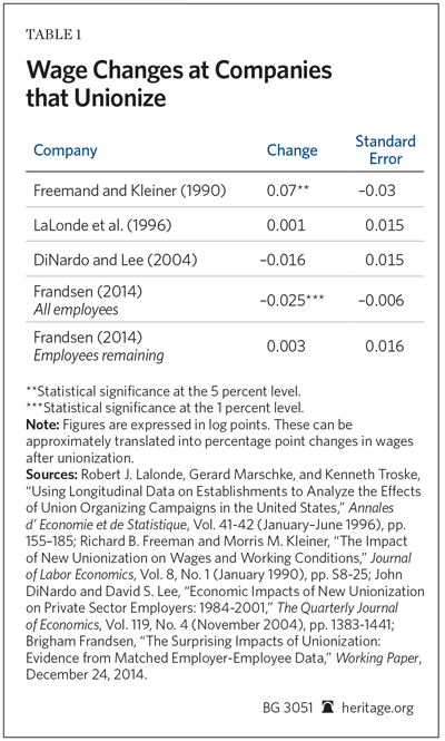
Union organizers disproportionately target large, high-productivity companies.[10] These companies also pay above-average wages. Many economists have analyzed whether unionizing causally increases wages. These studies compare pay at companies where workers vote to unionize with pay at similar companies whose workers vote against unionizing. These studies find little effect of unionizing on wages. Table 1 summarizes the results of the most recent studies.

One early study comparing 124 firms suggested that unionizing raised pay 7 percent.[11] Further studies examining more firms found no statistically detectable effect.[12] Researcher Brigham Frandsen discovered a source of bias in these earlier studies. He corrected it and examined virtually every firm whose employees voted on unionizing since 1980. He found that average pay falls 2.5 percent at newly organized firms.[13] This surprising result occurs because many highly paid workers quit their jobs after their companies unionize—reducing average wages. Frandsen found that unionizing had no effect on pay for workers who stayed with their firm. Such limited effects on wages seem a weak justification for forcing workers to pay union dues.

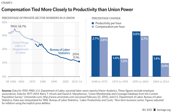
Pay and Productivity. Productivity has a much bigger impact on pay than does union power. In the post-war era, workers’ compensation growth has closely tracked productivity growth—and had little relationship with union membership. Chart 1 shows this visually.

From 1948 to 1973, both pay and productivity grew at almost 3 percent a year, while union density fell by one-fifth. Over the next two decades, productivity growth dropped to 1.4 percent a year. Pay growth similarly fell to 1.2 percent annually. During this time union membership continued to decline.

 

In the late 1990s and early 2000s, productivity returned to 3 percent annual growth. Union density continued to fall. Compensation growth did not. It followed productivity growth and surged to almost 3 percent a year. From 2004 onward, both productivity and pay growth have slumped, as has union membership. Workers’ pay rises when they become more productive—not when unions have more power. Policymakers who want to increase wages should look for ways to help workers become more productive or use their existing skills more effectively.

Right-to-Work Laws

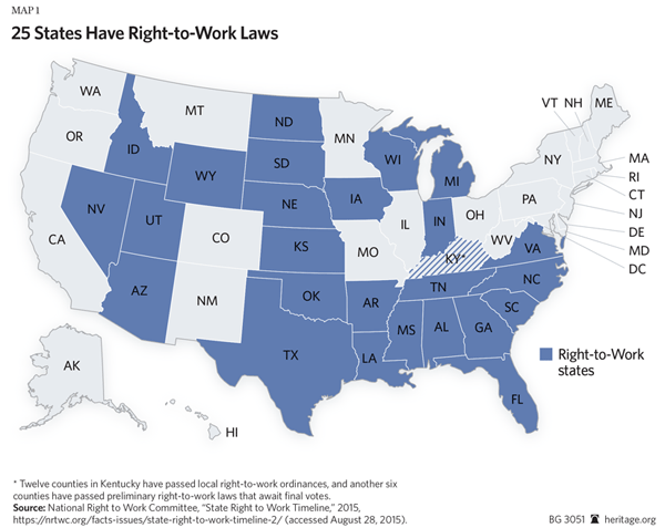
Right-to-work laws present a natural economic test of unions’ economic impact. The National Labor Relations Act (NLRA) allows unions to negotiate contracts that require companies to fire workers who do not pay union dues. The NLRA also allows right-to-work laws that prohibit these provisions. Twenty-five states have passed right-to-work laws, and have voluntary union dues. Workers in non-RTW states must pay dues or they will be fired. Unsurprisingly, unions have far more members in non-RTW states.

If unions raise living standards, workers in non-RTW states should have higher wages, after controlling for other factors like education and living costs. If states with compulsory dues do not have higher wages, this strongly suggests that expanding union membership does little to raise living standards.

 

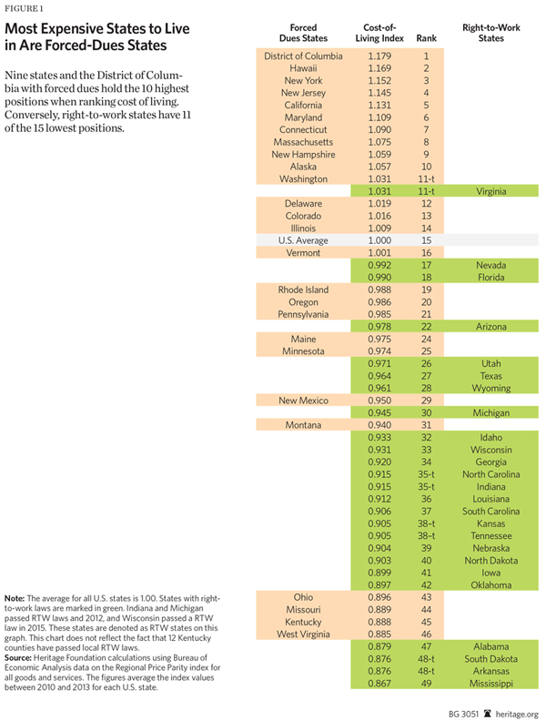
Right-to-Work States Have Lower Living Costs. Examining this question is more complicated than it might appear. Unions often point out—accurately—that average wages in right-to-work states are below those in non-RTW states.[14] But right-to-work states also have below-average living costs. Virtually the entire South has passed RTW; no Northeastern states have. The Northeast has higher costs of living and higher average wages; the South has lower living costs and lower wages. The higher wages in non-RTW states do not necessarily purchase more goods and services.

Figure 1 shows this visually. It displays average living costs from 2010 to 2013 for each U.S. state. The values show how much more or less goods and services cost in particular states relative to the U.S. average. For example, New Yorkers pay 15 percent more than the average American, and Alabamians pay 12 percent less.

All but one state with living costs above the national average impose compulsory dues. Conversely, 16 of the 20 states with the lowest costs of living have RTW laws.

 

Wages move one-to-one with cost-of-living differences, after accounting for worker characteristics and local amenities.[15] Consequently, economists need to account for differences in living costs when examining how right-to-work laws affect real wages.[16]

Previous Research on Right to Work and Wages. Most economists who account for cost-of-living differences find that right-to-work laws have little effect on real pay. William Moore summarizes the academic literature and concludes:

The empirical evidence accumulated in the 1970s and 1980s indicates that RTW laws do not have strong lasting effects on wages. Most researchers find that RTW laws have no impact on union wages, nonunion wages, or average wages in either the private or public sector.[17]

W. Robert Reed re-examined the question and found that—after controlling for economic conditions when states passed right-to-work laws—workers in RTW states have higher wages than in states with compulsory union dues.[18]

More recently, Economic Policy Institute researchers came to the opposite conclusion. In a 2011 report, Elise Gould and Heidi Shierholz used regression analysis to compare workers in right-to-work states and states with mandatory union dues. They found that controlling for living costs only partially closes the wage gap between RTW and non-RTW states. They concluded that comparable workers earn approximately 3 percent lower real wages in right-to-work states.[19]

In 2015 testimony before the Wisconsin legislature, this author replicated Gould and Shierholz’s study and found problems with that analysis.[20] Sherk found that the Gould and Shierholz model did not fully control for living costs, and suffered from biases caused by measurement error. Sherk also argued that Gould and Shierholz included improper control variables. Sherk adopted an alternative model specification correcting for these problems and found no difference in real wages between RTW and non-RTW states.

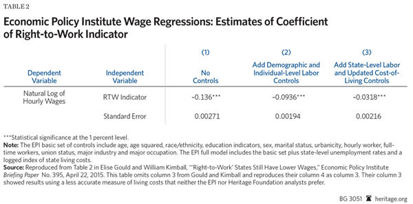
In a recent report, Gould and a new co-author, William Kimball, respond to these criticisms. They argue that only “non-standard specifications of wage equations can move the estimated RTW penalty to statistical insignificance.… [T]he regression specification that Sherk (2015) constructs to find no RTW wage differential looks deeply data-mined.”[21] Table 2 reproduces their main findings.

As Table 2 shows, Gould and Kimball find that average wages are approximately 13 percent lower in right-to-work states.[22] Controlling for demographic factors and labor-market factors reduces that gap to approximately 9 percent. After adding living costs and state unemployment rates as control variables, the gap remains a statistically significant 3.2 percent. On this basis Gould and Kimball conclude right-to-work laws lower wages 3 percent. Unions have used this finding to argue that legislators in Missouri and other states should force workers to pay union dues.

A Response to the Critics

Gould and Kimball accuse Sherk of “extensive searching for the model that produces the result he wants.” Data-mining is often a legitimate concern. Econometricians can frequently find some combination of control variables that produces a desired result. To demonstrate that such data-mining does not drive the CDA’s results this Backgrounder adopts the same control variables as Gould and Kimball.

This Backgrounder replicates their work and demonstrates that two analytical choices drive their conclusion that right-to-work laws lower wages: (1) using an econometric model that only partially controls for living costs, and (2) examining private-sector and government employees together instead of separately. Correcting for these problems shows that right-to-work laws have no statistically significant effect on real private-sector wages. State and local government employees do earn approximately 5 percent less in right-to-work states.

CDA analysts still consider some of EPI’s economic control-variable choices to be problematic. Appendix B shows results using the CDA’s preferred model. Removing potentially endogenous variables and including controls for metropolitan population size shows that private-sector workers have slightly, but statistically significantly, higher real wages in right-to-work states.

Data and Methodology

Like Gould and Shierholz (2011), Sherk (2015), and Gould and Kimball (2015), this Backgrounder uses data from the Census Bureau’s Current Population Survey (CPS). The Census Bureau makes this data publicly available. However, researchers—including Gould and Kimball—often make data-quality adjustments to correct for known problems.[23] This author would have preferred to use EPI’s data to avoid any implication that idiosyncratic CDA adjustments explained these results. However, EPI ignored repeated requests to share its data and code. Consequently, the CDA used adjusted CPS data made publicly available by another liberal think tank, the Center for Economic Policy Research (CEPR). CEPR developed this data with the assistance of EPI researchers.

Both this Backgrounder and Gould and Kimball use regional price parity (RPP) data from the Bureau of Economic Analysis to estimate cost-of-living differences. Appendix A discusses these data sources in greater detail.

Both the Heritage and the EPI reports use regression models that compare differences in the log of workers’ wages, controlling for the influence of other variables—including right-to-work status. The regression model is:

Yi= α + γRTWi + βXi + εi

Where Yi represents the log of individual real wages, α is a constant, RTWi is a dummy variable indicating if the individual lives in a right-to-work state, Xi is a vector of additional control variables, and εi is an error term. The coefficient on γ indicates the effect that RTW laws have on wages. This report uses the same control variables that Gould and Kimball used in their preferred specification. Those are:

• Union status;[24]
• Five mutually exclusive categories of racial/ethnic background—(1) white, (2) black, (3) Hispanic, (4) Asian, or (5) other;
• Six educational categories—(1) high school dropout, (2) high school graduate, (3) some college, (4) associate’s degree, (5) bachelor’s degree, or (6) advanced degree;
• Age and age squared;
• Gender;
• Four marital status categories—(1) never married, (2) married, (3) divorced or widowed, or (4) separated;
• Hourly or salaried employee;
• Full-time or part-time employee;
• Live in a metropolitan area or not;
• State unemployment rate;
• Major industry and occupation group; and
• Log of the regional price parity cost of living index.

 

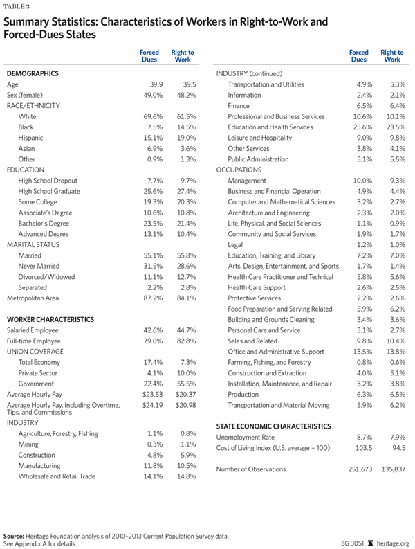
Table 3 summarizes how these variables differ for workers in RTW states and in states with compulsory dues. While similar in many respects, RTW states and non-RTW states have notable differences. Workers in RTW states are slightly more likely to have a salaried instead of hourly job, to work full-time, and to have a job instead of being unemployed.

Workers in right-to-work states are also significantly less likely to belong to a union or to be covered by a collective bargaining agreement. While 17 percent of workers in states with compulsory dues are represented by a union, 7 percent belong to unions in states with voluntary dues. Only 4 percent of private-sector workers in right-to-work states are represented by a union while 10 percent do–two and a half times as many—in states with compulsory dues.

Notably, right-to-work states have both lower costs of living and lower hourly wages. Workers in RTW states earn $3.16 an hour less than workers in non-RTW states. The average worker in a right-to-work state also enjoys living costs 5.5 percent below the national average. Workers in states with compulsory dues pay 3.5 percent more than the national average. Analysts need to conduct more thorough analysis before concluding that workers in right-to-work states have less purchasing power.

Results

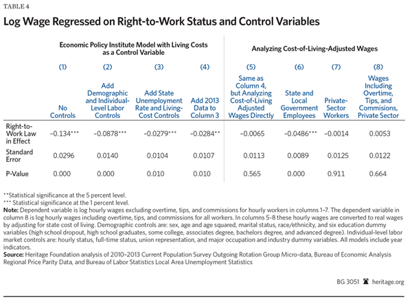
Replicating the EPI Analysis. Table 4 presents the main results of the CDA’s regression analysis. Columns 1 through 4 attempt to replicate Table 2 of Gould and Kimball.[25] Column 1 shows that workers in RTW states have approximately 13 percent lower wages than workers in other states, if analysts ignore all other factors.[26] Column 2 adds demographic and individual-level labor market variables to the analysis. This reduces the right-to-work coefficient to approximately 9 percent. Column 3 shows EPI’s preferred specification, which adds the log of state living costs and the state unemployment rate. This reduces the estimated right-to-work coefficient to a statistically significant –2.8 percent. Column 4 adds 2013 data—Gould and Kimball examined data only from 2010 to 2012.[27] This has virtually no effect on the results.

The CDA found results somewhat different from the EPI estimates reproduced in Table 2. Despite using the same underlying data, model, and control variables as Gould and Kimball, the coefficients in Table 4 all show slightly smaller effects of RTW laws. CDA analysts attempted to investigate the source of this discrepancy. Unfortunately, this proved impossible as Dr. Gould did not respond to repeated requests to share her data and code. However, the differences between the EPI-adjusted CPS and CEPR-adjusted CPS data are small. They appear unlikely to affect the qualitative conclusions of the Heritage or EPI analyses.

EPI Only Partially Accounts for Cost-of-Living Differences. The Economic Policy Institute’s preferred specification has a major problem: It only accounts for three-quarters of the difference in living costs between states. The appendix in Gould and Kimball reports the coefficient on the living cost variable as 0.771. Heritage’s replication finds a similar coefficient: 0.722. In economic terms, this means that the EPI model expects workers in states with 10 percent below-average costs of living to have between 7.2 percent and 7.7 percent—not 10 percent—lower wages.[28] This partial adjustment for living costs seriously biases EPI’s results.

To see this, consider how the EPI model treats RTW state Iowa. Chart 2 shows that in Iowa, goods and services cost about 10 percent below the national average. Across America, wages move almost one-for-one with cost-of-living differences, after accounting for differences in local amenities.[29] Consequently, Iowa will also have about 10 percent below average nominal wages. But the EPI model explains only about 7 percent of this lower nominal pay. So Iowans appear to earn wages 3 percent below the national average in the EPI model, despite these lower wages being fully offset by lower costs of living. EPI’s model will attribute part of these unexpectedly low earnings to other variables—such as right-to-work laws—correlated with low living costs. The EPI model does not fully account for differences in purchasing power. This biases their estimates toward finding lower wages in RTW states.

Measurement error in the cost-of-living index may explain this dynamic. Although the RPP index measures living costs better than previous indexes, it has some shortcomings. Besides the classical sampling error that any survey contains, the RPP does not sample rural areas but assigns them prices from nearby urban areas.[30] Prices in rural Pennsylvania probably differ significantly from prices in Pittsburgh and Philadelphia. Consequently, the RPP measures living costs with error.

Such measurement error has well-known statistical properties: measurement error in control variables (for instance, living costs) biases regression estimates toward zero, while measurement error in dependent variables (for example, wages) reduces statistical precision but does not bias the results.[31] Measurement error would make living costs appear to have less of a relationship with wages than they actually do.

Fully Accounting for Living Costs. Adjusting wages for cost-of-living differences and then running the analysis corrects this problem. This fully controls for living cost differences. It also moves the measurement error from one of the control variables to the dependent variables (real wages). This increases the model’s margin of error but does not bias the estimates. Table 4, column 5, shows the results of analyzing real wages directly instead of including the cost-of-living index as a control variable.

Analyzing real wages directly eliminates almost the entire negative correlation between right-to-work laws and wages. The estimate falls from 2.8 percent lower wages in RTW states to a statistically insignificant –0.7 percent. The specification in column 5 uses the same control variables that Gould and Kimball used. It differs only by analyzing real wages instead of nominal wages. Completely controlling for price differences eliminates the negative effects of right-to-work on wages that EPI reported.

 

Sherk (2015) also analyzed real wages and found similar results.[32] Gould and Kimball did not attempt to replicate this finding in their response. The Economic Policy Institute’s researchers either did not analyze cost-of-living-adjusted wages, or they did and withheld these results.[33] Neither possibility should inspire confidence in the robustness of their findings. The model that is robust to measurement error and fully controls for living costs shows that right-to-work laws have little effect on real wages.

Some economists, such as Michael DuMond, Barry Hirsch, and David Macpherson, do suggest including living costs as a control variable.[34] They argue that differences in amenities between cities mean that nominal wage differences should not fully offset cost-of-living differences. Winters shows that measurement error biases these results. He demonstrates that wages move one-for-one with living costs if researchers directly control for amenities and use econometric methods to correct for measurement error.[35] Appendix C shows that implementing this approach produces very similar results to those presented in Table 4. Workers have the same purchasing power in RTW states and states with forced dues.

Private Sector vs. Government

Right-to-work laws theoretically affect wages differently in the private sector than in government. Private-sector unions argue that RTW reduces union membership and thus their ability to raise wages. Conversely, right-to-work laws can attract investment, which increases the demand for labor.

Government unions affect wages quite differently. They raise their members’ pay through political leverage. Government unions devote a large portion of their budgets to political activism. For example, the American Federation of State, County, and Municipal Employees (AFSCME) national headquarters spent a third of its $200 million budget on politics and lobbying in election year 2014.[36] By using their resources to elect political allies, government unions can control both sides of the negotiating table. This enables them to win generous concessions that private employers would rarely accept. Right-to-work laws reduce the resources government unions can use to help elect their political allies—potentially reducing government pay.

Because RTW affects wages through different channels in the government and private sector, analysts should examine these sectors separately. Table 4, columns 6 and 7 repeat the specification of column 5 for state and local government employees and private-sector workers.[37]

Column 6 shows that state and local employees earn approximately 5 percent lower wages in right-to-work states. Voters and policymakers should see this as a benefit of right-to-work laws. State government employees in all but five states earn more than similarly skilled private-sector workers.[38] Private-sector workers should not pay excessive taxes so that government employees can enjoy higher standards of living than they do.[39]

Column 7 shows that right-to-work laws have an even smaller impact on private-sector wages than on the economy overall. Private-sector workers earn a statistically insignificant 0.1 percent less in RTW states than in non-RTW states.

Overtime, Tips, and Commissions. Column 8 shows a final specification. Gould and Kimball used a measure of wages that excludes overtime, tips, and commissions from hourly employees’ pay. This ignores a significant component of many employees’ pay. Such variable compensation has become an increasingly large part of workers’ compensation over the past generation.[40]

Column 8 shows the same specification as column 7, with the exception that it includes overtime, tips, and commissions in hourly workers’ pay.[41] The more inclusive definition of compensation reverses the sign of the RTW coefficient. Using it shows that right-to-work laws are associated with (statistically insignificant) 0.5 percent higher private-sector wages. EPI’s negative conclusions about RTW are highly sensitive to alternative model specifications.

Unions Affect Average Private-Sector Wages Little. Gould and Kimball argue that “RTW laws seek to hamstring unions’ ability to help employees bargain with their employers for better wages, benefits, and working conditions.” If that is the case, RTW laws are wholly ineffective. Many workers opt out of union membership when union dues become voluntary. Nonetheless, real wages in right-to-work states are just as high for private-sector workers as in states with compulsory dues.

The fact that workers in states with compulsory union dues do not have detectably higher purchasing power strongly suggests that unions do not promote general prosperity. It also shows that policymakers have no economic justification for forcing workers to pay union dues. Workers who want to unionize have the right to do so. But the government should not force workers who see little benefit from union representation to pay for it.

Right-to-Work States Have Lower Unemployment. While right-to-work laws do not affect average private-sector wages, they do affect job creation. Unions organize more aggressively in non-RTW states.[42] Most companies want to avoid being unionized. Consequently, many businesses prefer to locate in right-to-work states.

This does not, of course, apply to all companies. Highly skilled employees typically have little interest in general representation. Few technology-sector workers, for example, want the seniority-based raises and promotions that unions typically prefer to performance-based pay. Consequently, right-to-work laws do little to attract companies that employ highly skilled workers. Many other companies do pay close attention to states’ RTW status—especially manufacturing companies. David Brandon, president of the Pathfinders, an economic development consulting firm, explains:

About 35-to-40 percent of manufacturing enterprises in the automotive industry insist on operating in a right-to-work state. Another 20-to-25 percent say it is a very important factor and will be used as a second- or third-tier factor in site selection. More than half of our companies either make it a threshold or a very important factor in making a decision on where to locate a factory and other operations.[43]

The city of Bowling Green in Warren County, Kentucky, provides an informative case study. In December 2014, Warren County passed a local RTW ordinance using its Home Rule powers. Over the next six months, 47 separate economic development projects approached local officials and expressed interest in locating the county.[44] Right-to-work attracts many companies that will not locate in states with compulsory dues.

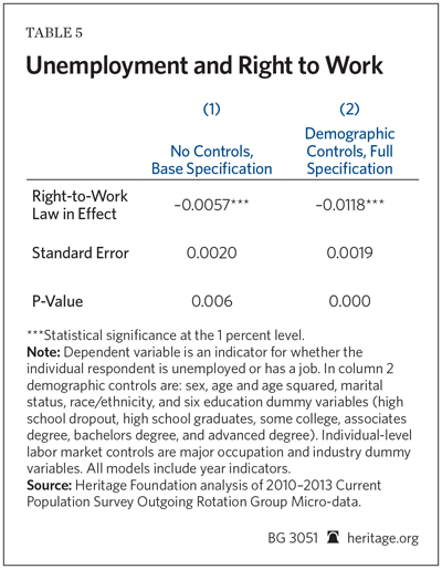
Rigorous econometric studies generally come to the same conclusion. Moore writes in his literature survey that the “stronger methodological studies…find that RTW laws have a significant, positive influence on industrial growth and economic development.”[45] Gould and Kimball disagree, and cite several studies finding small effects of right-to-work laws on employment.[46] There is a tension in their arguments: They contend that unions significantly raise labor costs, but that businesses ignore these higher costs when deciding where to locate.[47] A natural test of their argument is to examine how unemployment rates—not just wages—differ between RTW and non-RTW states.[48] Table 5 shows this analysis.

 

The first column of Table 5 shows the results of regressing a RTW variable on the probability that individual workers are unemployed. Without controlling for any other factors, workers in right-to-work states have 0.6 percentage point lower unemployment rates. Column 2 expands the analysis to include the control variables used in Gould and Kimball’s preferred specification in Table 2, except for those questions that the CPS only asks employed workers.[49] This model shows that workers in RTW states have 1.2 percentage point lower unemployment rates than workers in states with compulsory dues.

The same model that Gould and Kimball used to analyze the effects of right to work on wages shows much lower unemployment in RTW states. State legislatures can make it easier for the unemployed to find jobs by passing right-to-work laws.

Conclusion

The labor movement and its allies argue that expanding union membership would raise wages for most workers. However—unions operate as labor monopolies. They raise wages for their members by raising prices and reducing job opportunities for non-union workers. They do not increase average wages overall.

The experience of right-to-work states shows this clearly. Right-to-work laws make union dues voluntary. Unions organize less aggressively and have much lower membership in RTW states. However, private-sector workers have the same real wages in RTW as in non-RTW states. Compulsory dues and high union membership do not raise real wages in the private sector. In order to raise wages, policymakers should focus on measures to help workers increase their productivity or reduce barriers to using their existing skills.

—James Sherk is Research Fellow in Labor Economics in the Center for Data Analysis, of the Institute for Economic Freedom and Opportunity, at The Heritage Foundation.

Appendix A: Methods and Data

The Center for Data Analysis used outgoing rotation group data from the Current Population Survey (CPS) to measure workers’ hourly earnings and demographic characteristics. The Census Bureau makes raw CPS data publicly available online for download. However, researchers often adjust CPS data to correct for factors such as top-coding, in which the Census Bureau censors the income responses it publicly releases. Gould and Kimball used such adjusted CPS data.[50] The CDA would have preferred to use their data. This would have demonstrated that differences in model specification—not selective data adjustments—drive the differences between their results and those presented in this paper.

The Economic Policy Institute (EPI) did not respond to the CDA’s repeated requests to share their data and code. Consequently, the CDA used adjusted CPS data made publicly available by another prominent left-wing think tank, the Center for Economic and Policy Research (CEPR).[51] CEPR created its CPS extracts with the assistance of EPI researchers. The CEPR data adjustments are very similar to those that Gould and Kimball made. No one can seriously accuse CEPR of selectively adjusting CPS data to produce conservative results. However, as Tables 2 and 4 demonstrate, even using the CEPR data, the CDA could not replicate the EPI results exactly.

The CDA’s use of CEPR data when replicating EPI analysis does not imply CDA endorsement of all CEPR choices in cleaning the raw CPS data. For example, CEPR used the Consumer Price Index Research Series (CPI-U-RS) to adjust wages for inflation. Like the Congressional Budget Office and the Federal Reserve, Heritage’s CDA considers the Personal Consumption Expenditures (PCE) price index a more accurate measure of inflation. Had this not been a replication, the CDA would have used the PCE deflator.[52]

The CDA used the CEPR variable “rw” for the wage analysis in columns 1 through 7 in Table 4. This variable measures salaried employees’ hourly wages by dividing their usual weekly earnings by their usual weekly hours worked. It measures hourly employees’ wages by using their reported hourly wage. Column 8 in Table 4 uses the CEPR variable “rw_ot,” which measures hourly employees’ wages using the same method as for salaried employees. This includes overtime, tips, and commissions, which are excluded from reported hourly wages. CDA analysts expressed both wage and regional price parity data in logs. Following researchers Barry Hirsch and Edward Schumacher, the CDA analysts excluded workers with imputed wages.[53]

The Census Bureau conducts the CPS using a multi-stage stratified sampling design. Failure to account for this design will cause researchers to underestimate standard errors. Both Sherk (2015) and Gould and Kimball (2015) made this mistake. CEPR and others note that researchers can closely approximate the CPS stratified sampling design by creating a primary sampling unit variable that groups respondents by city size (cbsasize) and consolidated statistical area (cmsacode). They can then estimate standard errors stratifying by cmsacode and using the new variable as their primary sampling unit.[54] The CDA followed this methodology throughout this Backgrounder. Analysts also used heteroscedasticity-robust standard errors.

CDA analysts used regional price parity (RPP) data produced by the Bureau of Economic Analysis to measure living cost differences. The RPP is a newly produced dataset available at the state and metropolitan statistical area (MSA) level. RPP data is currently available from 2008 through 2013.

For the analysis in Tables 2 through 4, CDA analysts matched RPP to CPS data at the state level. For the analysis in Appendix Tables C.1 and C.2, they matched RPP to CPS data at the MSA level.[55] The CPS uses 2003 MSA definitions, while the RPP uses 2013 MSA definitions. CDA analysts excluded from this match any MSAs whose definitions changed between 2003 and 2013. Many workers also live outside MSAs. In total, approximately 61 percent of the observations matched to RPP at the statewide level were also matched at the MSA level.

CDA analysts used the same data sources as Winters (2009)[56] to construct the MSA-level amenity variables:

• Oceans. CDA analysts consulted maps to determine if any counties in a MSA bordered the Atlantic or Pacific Oceans or the Gulf of Mexico. If so, that MSA was coded as bordering that ocean.
• Climate and topography. CDA analysts used the Department of Agriculture’s Economic Research Service’s Natural Amenities Scale for county-level data on average January and July temperatures, average January sunlight and July humidity, percentage of water area, and topographical features.
• Air pollution. CDA analysts used Environmental Protection Agency data for 2011–2013 average county-level ozone parts per million and annual particulate matter (2.5).
• Crime. CDA analysts used data from the USA Counties website formerly maintained by the U.S. Census Bureau. The Census Bureau has discontinued this program and its data runs through 2008. It seems unlikely that relative county-level crime rates have diverged substantially in the two to five years after the data ends. Consequently, CDA analysts used average 2007–2008 county-level property crime and violent crime rates.
• Unemployment. CDA analysts obtained annual state and county-level unemployment rates from the Bureau of Labor Statistics’ Local Area Unemployment Statistics program for 2010–2013.

CDA analysts omitted one variable that Winters included: average commuting time. This data comes from the American Community Survey (ACS), which does not record the MSA of residence for respondents. Rather, the most precise geographic locator available is Public Use Microdata Areas (PUMAs)—which often do not align with MSA boundaries. The CDA omitted this variable rather than attempt to match ACS commute time data at the PUMA level to CPS data at the MSA level with potentially large errors. CDA analysts did not compile the ACS data and has no reason to believe that adding commute time would change the result shown here.

The CDA constructed MSA-level amenities variables from county-level data by taking a weighted average of the county-level data, using as weights the population of each county in the MSA containing data on that variable.

In 2012, both Indiana and Michigan passed right-to-work laws. CDA analysts included these states in the analysis and classified them as non-RTW states until these laws took effect. After they did so, CDA analysts excluded Michigan and Indiana observations from the analysis. Less than two years seems too soon for these laws to have a significant effect on wages in either state.

Appendix B: Alternative Control Variables

Throughout the main text of this Backgrounder, The Center for Data Analysis used the control variables in Gould and Kimball (2015) and in Gould and Shierholz (2011). This was done to demonstrate that incompletely controlling for living costs and combining government and private-sector workers—not the choice of other control variables—drove the findings that RTW laws lower wages.

CDA analysts believe that several of EPI’s economic control variables are inappropriate to include: industry, occupation, full-time versus part-time and hourly versus salaried status, state unemployment rate, and union membership. Right-to-work laws affect wages in part by influencing these variables. Many states pass right-to-work laws with the intention of attracting businesses and better jobs. Increased employment also puts upward pressure on wages and working conditions. Montgomery, Alabama, has more full-time and manufacturing workers and lower unemployment precisely because Alabama’s right-to-work law helped to induce Hyundai to locate there instead of in Ohio. Similarly, unions argue that right-to-work laws reduce their membership, and thus the availability of good jobs.

Including these variables holds constant the channels through which right-to-work laws affect wages. While these may be sensible control variables in other contexts, analysts investigating the causal effect of right-to-work laws on wages should not include them.

CDA analysts also believe that EPI should have included more detailed controls for city size than a single dummy variable for metropolitan areas. Over 80 percent of CPS respondents report living in a metropolitan area. This provides limited identifying variation. The CPS also contains more detailed information on overall metropolitan area size. Larger metropolitan areas have greater economies of scale and network effects. This can substantially increase worker productivity and wages. An extensive literature has examined the nature of these “agglomeration economies.”[57] Since the non-RTW Northeast has a substantially higher population density than the predominantly RTW South and West, ignoring agglomeration economies could potentially bias the EPI model.

Changing the model to exclude potentially endogenous variables and include more detailed controls for city size significantly impacts the results. Under the CDA’s preferred specification, the right-to-work coefficient for private-sector workers becomes positive and significant at conventional levels. Gould and Kimball’s preferred control variables underestimate the positive effects of right-to-work laws.

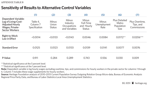
Table 3 in Gould and Kimball displays their robustness tests. They show that removing each variable individually has a small effect on their overall results. They do not show the cumulative effect of these control variables on their analysis. Appendix Table B in this Backgrounder shows the cumulative effect of these modeling choices.

Column 1 of Table B shows the same specification in column 7 of Table 4. The dependent variable is hourly wages for private-sector workers, converted from nominal into real dollars using the RPP index of state living costs and the CPI-U-RS. All other control variables follow Gould and Kimball’s specification: age and age squared, sex, marital status, race/ethnicity, the six education dummy variables, hourly status, full-time status, union representation, and major occupation and industry dummy variables. All models include year indicators.

Under this specification, RTW laws are associated with statistically insignificant –0.1 percent lower wages for private-sector workers. Column 2 removes the union status variable. This decreases the coefficient on the right-to-work variable to a statistically insignificant –1.3 percent. This Backgrounder draws the conclusion that unions do not raise wages in the private sector. It is worth noting that removing union status from the control variables has no effect on that conclusion.

Column 3 then removes both industry and occupation variables from the analysis. It confirms Gould and Kimball’s finding that these variables have little effect on the analysis. The coefficient on the RTW variable drops slightly to a (statistically insignificant) –1.4 percent.

Column 4 removes the full-time versus part-time and salaried versus hourly dummy variables. This has a substantial effect on the estimates—increasing it to +0.5 percent. However, the RTW variable remains insignificant at conventional levels. Column 5 removes the statewide unemployment rate from the analysis. This has a modest effect, increasing the coefficient on the RTW variable to a—still statistically insignificant—+0.8 percent.

Column 6 adds controls for detailed metropolitan area population size. This increases the RTW coefficient to 1.7 percent. Under this specification, the RTW coefficient is statistically significant at the 3 percent level. More defensible control variables show that workers have higher real wages in RTW states.

Column 7 makes one more change, using the definition of wages that includes overtime, tips, and commissions for hourly workers. This increases the RTW coefficient to 2.1 percent. This estimate is statistically significant at the 1 percent level.

EPI’s preferred control variables suffer from serious endogeneity concerns. Pointing out that other authors have used these variables elsewhere does not make them any less endogenous when studying right-to-work laws.

It is worth noting the implications of the effects of removing the individual-level economic controls from the analysis. Union members have higher wages than non-union members (though this may not be causal). The fact that including union membership in the analysis increases the RTW coefficient indicates that RTW states have lower union membership. Ignoring the relationship between this lower union membership and average wages makes wages in RTW states look higher.

Similarly, including the unemployment rate, full-time versus part-time and salaried versus hourly coefficients all reduce the coefficient on the RTW variable. This implies that RTW states have lower unemployment rates and a greater proportion of full-time and salaried jobs than non-RTW states. (The summary statistics in Table 3 show that this indeed occurs.) These are all signs of stronger demand for labor in RTW states. This suggests that RTW laws have beneficial economic effects—effects that the EPI model ignores.

Finally, Gould and Kimball objected to Sherk’s inclusion of detailed educational attainment, marriage and sex interaction terms, and controls for parent and single-parent status. They cite the inclusion of these variables as evidence of data-mining. CDA analysts simply converted the main CPS education variable into an interaction term.[58] This used all the available information contained in the CPS responses. CDA analysts believes that a sex and marriage interaction term is important given the fact that marriage is generally associated with a larger earnings effect for men than for women.[59] Researchers have also identified single parenthood as a significant factor impeding economic mobility.

However, including these variables has little effect on the results. Robustness tests (not presented here) show that using all the information on educational attainment or using the EPI’s six education categories makes no difference in the results. Including the marriage/sex interaction term and the parenthood and single-parent controls increases the coefficient on RTW by less than 0.4 percentage points in Column 7 of Table 4. Differences in how to control for cost of living, and combining private-sector and government employees—not differences in detailed control variables—drive the disparity between Gould and Kimball and the results presented in this Backgrounder.

Appendix C: Modeling Living Costs as a Control Variable

Both Gould and Shierholz (2011) and Gould and Kimball (2015) use living costs as a control variable instead of directly analyzing living-cost-adjusted wages. Their full regression results show (and this report confirms) that this only adjusts for about three-quarters of differences in living costs among states.

DuMond, Hirsch, and Macpherson (1999) advocate making just such a partial adjustment for living-cost differences. They argue that different areas have different amenities that affect pay that economists do not capture in standard wage analyses. For example, Los Angelinos may accept lower wages in exchange for enjoying California’s temperate climate and living near the beach. Workers in Bismarck, North Dakota, may require higher wages to persuade them to endure frigid winters and sparse population. DuMond and his co-authors argue that including living costs as a control variable appropriately captures the effect of differences in amenities on wages.

Winters points out that measurement error in the cost-of-living variable will bias its coefficient toward zero, improperly underestimating the effect of living costs on wages. He also argues that if amenities affect wages, researchers should control for them directly. He suggests correcting for measurement error by instrumenting the price index for all goods and services with lagged values of the price index for rental costs (which suffers only from classical survey measurement error). He shows that after implementing this correction and controlling for amenities directly, living costs move one-for-one with differences in average hourly wages.

Sherk (2015) showed that RTW laws have no correlation with living-cost-adjusted wages in statewide analysis. Sherk also showed that following Winters’s methodology and controlling for several statewide amenities eliminates the apparent negative correlation between right-to-work laws and wages.

Gould and Kimball make a reasonable objection to this specification. They point out that Sherk included amenities variables that only make sense at the local level—not statewide—such as bordering an ocean or average January temperatures. Workers in Fresno, California, will not accept lower wages on the grounds that Los Angeles residents enjoy easy access to the beach. Workers in New York City will not demand higher pay because lake-effect snow hammers upstate Buffalo. Gould and Kimball show that using instrumental variables to correct measurement error but not accounting for amenities has only a small effect on their results.

While arguing against measuring statewide amenities makes sense, the resulting Gould and Kimball model does not. If they believe that differences in amenities affect wage rates, they should include them in their analysis. If they believe that amenities do not significantly affect wages, they should adjust for living costs directly. Their model with living costs as a control variable implicitly assumes that amenities are an important determinant of wages but nonetheless ignores them.

CDA analysts tested the robustness of the results presented in Table 4 by modeling living costs as a control variable and including controls for local amenities. They controlled for amenities at the metropolitan statistical area level and used MSA-level RPP living cost data. To avoid any appearance of data mining, CDA analysts used the same amenities variables as Winters (2009), with the exception of average commute time, which matches to MSA-level data only with considerable error. Appendix A discusses the data sources used and construction of the MSA-level variables in greater detail. The CDA controlled for the following amenities:

• Geography. Whether an MSA borders the Atlantic or Pacific Oceans or the Gulf of Mexico; the percent of landmass in the MSA covered by water; and five different topography variables (1) plains, (2) tablelands, (3) plains with hills and mountains, (4) open hills and mountains, and (5) hills and mountains);
• Weather. Average temperature in January, average temperature in July, average sun received in January, average July humidity;
• Crime. Average property and violent crime rates;
• Pollution. Average particulate matter (2.5) and average ozone parts per million;
• Metropolitan area population size; and
• Local unemployment rate.

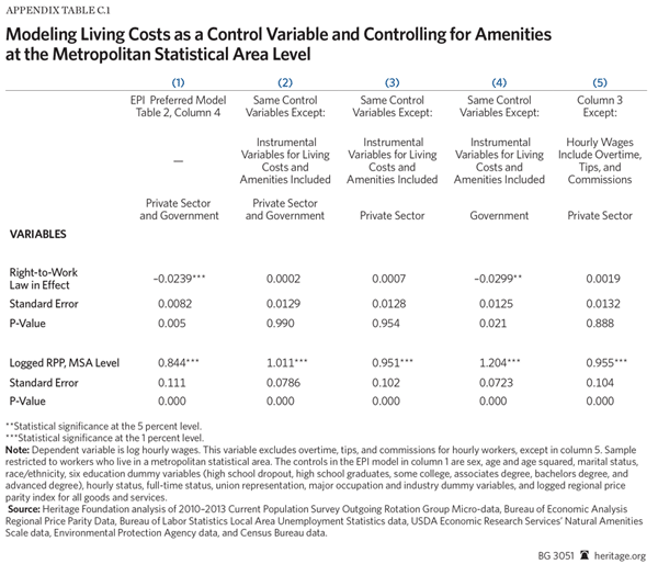
Appendix Table C.1 shows the results of this analysis. Column 1 shows the results applying the preferred Gould and Kimball (2015) specification from Table 4, Column 4 to the MSA-level data. Restricting the sample to respondents living in an MSA and using MSA-level price indexes slightly increases the value on their RTW coefficient from –2.8 percent to –2.4 percent. The coefficient on the living costs variable also increases from 0.72 to 0.84.

 

Column 2 implements the Winters methodology, controlling for measurement error using instrumental variables, and including the amenities controls. This change increases the coefficient on the RTW variable from –2.4 percent to 0.0 percent. Either adjusting for living costs directly, or including them as a control variable but controlling for other amenities that might affect wages, shows that right-to-work laws have little effect on wages.

Column 2 also replicates Winters’s main result: After researchers control for measurement error and observable amenities, wages move one-to-one with local living costs. The coefficient on the living-cost variable is statistically indistinguishable from 1.0. Including the Winters control variables is sufficient to explain the variation in wages dues to unmeasured amenities.

Columns 3 and 4 repeat this analysis for private-sector employees and state and local government employees, respectively. Relative to the overall sample, the RTW coefficient imperceptibly rises to 0.1 percent—statistically insignificant—for private-sector workers. For state and local government employees the coefficient falls to a statistically significant –3.0 percent wage penalty in RTW states.

Table 4, column 6, found that state and local government employees have approximately 5 percent lower wages in RTW states. The analysis incorporating amenities finds an effect roughly three-fifths that size. This may reflect the fact that controlling for amenities controls for one of the channels that facilitates rent-seeking by government unions. Jan Brueckner and David Neumark find that government employees are paid more in cities with desirable amenities.[60] Worker mobility limits the ability of local governments to raise taxes to increase their employees’ compensation. However, in areas with desirable amenities (such as beach access and pleasant weather) residents will accept higher taxes in order to enjoy those amenities. This gives government unions more ability to press for increased government pay (and thus taxes), transferring part of the value of those amenities to their members.

Column 5 repeats the analysis of column 3, only using the broader definition of wages that includes overtime, tips, and commissions for hourly workers. Unlike in Table 4, this has almost no effect on the results. The wage premium for private-sector workers in right-to-work states is a statistically insignificant 0.2 percent.

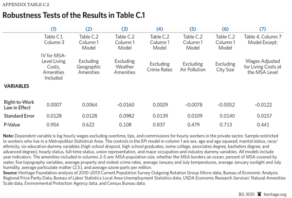
CDA analysts conducted robustness tests of the results presented in Appendix Table C.1. Appendix Table C.2 displays them. Column 1 repeats the base specification—using instrumental variables to estimate living costs, controlling for local-level amenities, and looking at private-sector workers—from column 3 of Table C.1.

Columns 2 through 6 show the results of re-estimating this model and iteratively dropping each of the categories of amenities: geography, weather, crime, air pollution, and city size.[61] In every case, the RTW estimates remain statistically insignificant. No single category of amenity control variables drives the finding that including amenities renders the RTW coefficient insignificant.

Column 7 shows the analysis after adjusting wages for living costs directly and without amenities. This corresponds to the specification in Table 4, column 7 only restricting the sample to respondents living in an MSA and using MSA-level living cost indexes. Doing so shows that private-sector wages are a statistically insignificant 1.2 percent lower in RTW states than in non-RTW states. This differs slightly from the results in Table 4 using statewide data. Further investigation showed that running the statewide analysis just on respondents living in an MSA produced similar results. The author conjectures that differences between the total population and the subsample of the population living in MSAs drive the differences between the results in Table 4 and Appendix Table C.2.

 

The EPI specification that shows a negative effect of right-to-work laws on wages has little theoretical justification. If researchers want to examine real wages, they should convert nominal dollars into real dollars before running their analysis. If researchers believe that differing local amenities drive differences in wages, they should include those variables in their analysis directly. Both of these approaches show that RTW laws have little effect on workers’ pay. The Economic Policy Institute only finds a negative relationship between RTW and wages by incorrectly accounting for differences in living costs.

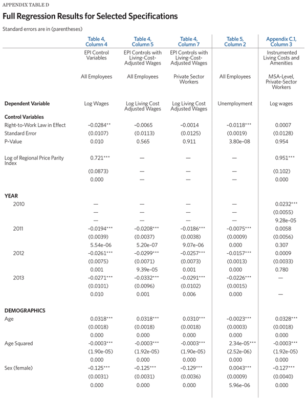
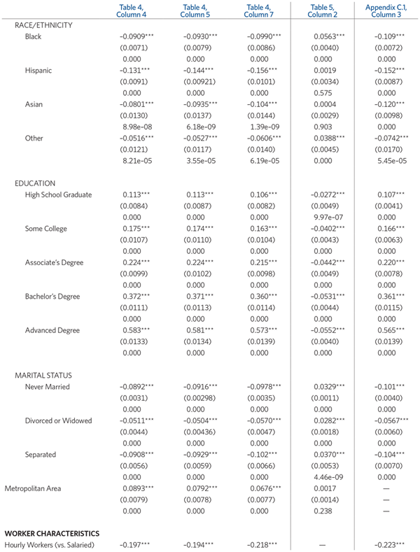
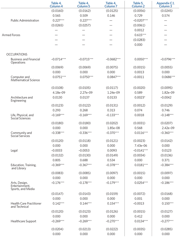
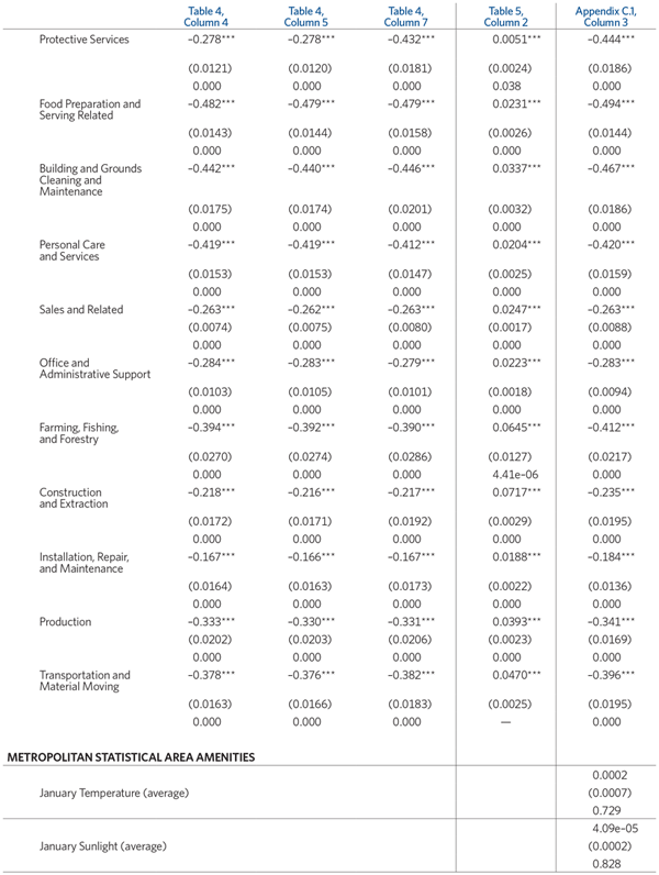
Appendix D: Full Regression Results

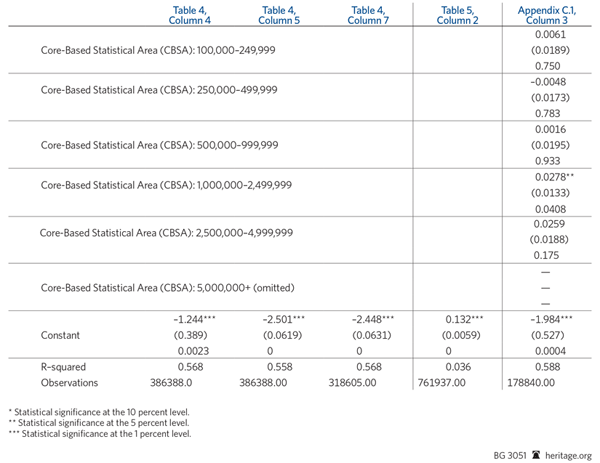
Appendix Table D shows the full regression results for several of the specifications presented in this paper: Table 4, column 4; Table 4, column 5; Table 4, column 7; Table 5, column 2; and Appendix Table C.1, column 3. The full results for any of the other tables, or the first-stage regression results from instrumental variables regressions are available from the author upon request.