Executive Summary
Between 2003 and 2006, home prices rose dramatically, but then they fell abruptly in 2007 and thereafter. While many believe that the main cause of the boom was easy access to credit in the form of subsidized interest rates, others have focused on different issues.
Clearly, economists are far from reaching a consensus on the roots of the boom-bust behavior in the real estate market. Some are skeptical about the role of interest rates; others conjecture that "irrational exuberance" played the most important role in shaping the housing boom. Many believe that mortgage securitization contributed to the rise of riskier loans; others have focused on the principal-agent problem, in which financial institutions have been unable to screen the loan applicants appropriately, and this lax screening has led to moral hazard.
This Special Report focuses on two government-sponsored entities (GSEs): the Federal National Mortgage Association (FNMA or Fannie Mae) and the Federal Home Loan Mortgage Corporation (FHLMC or Freddie Mac). Although these GSEs were established with the primary goal of developing a secondary mortgage market to increase homeownership among low-income groups and underserved areas, they became involved in profiteering and mortgage- backed securities (MBS), which left them far behind their primary goals.
This paper tries to capture the effects of GSE interventions in the housing market through subsidized interest rates and down payments on median single-family home prices at the national level. Contrary to the standard asset market model's approach, down payments may operate through two opposite transmission channels. The first channel affects the affordability for a typical home buyer; the second affects the supply of mortgage loans and may have positive effects on the demand side by increasing the resources available to homebuyers.
This analysis uses time series regression models with quarterly data from 1980 to 2010 to examine the effect of conventional 30-year mortgage interest rates and down payments on median home prices at the national level. It controls for such fundamentals as household assets, personal income, unemployment rate, property taxes, vacancy rate, and inflation expectations of home prices. The analysis demonstrates that:
- The conventional mortgage interest rate has a small negative impact on home prices.
- A 25-basis-point increase in the conventional mortgage interest rate, as discussed in a study by Scott Frame and Lawrence J. White, as a result of GSE liquidation and holding other things equal, leads to a 2.25 percent reduction in home prices. In other words, a jump in interest rates of 25 basis points has a small negative impact on home prices.
- While down payments have a negative association with home prices, the relationship is statistically insignificant for most models. However, in one of the estimated models, controlling for property taxes makes the down payment coefficient negative and statistically significant.
- A 25-basis-point increase in down payment leads to 1.5 percent lower home prices.
- The results of this study suggest that home prices are influenced more by mortgage interest rates than by down payments. This has important policy implications for financial institutions because changing the down payment compared to the mortgage interest rate will have less impact on home prices.
- Contrary to the expectations of policymakers, the Fannie Mae and Freddie Mac policy of easing requirements for purchasing homes since 1996 was found to be associated with a small rise in housing prices. The overall results indicate that home prices are influenced mainly by such fundamentals as household assets, personal income, and effective tax rates.
- The federal government's policy of subsidizing mortgage interest rates and lowering down payments to raise homeownership has failed due to inelasticity of home prices to mortgage interest rates and down payments.
- Indeed, the government's interventions in the market have led to a huge amount of deadweight loss for society rather than helping low-income individuals secure homeownership through lower prices. Although lower interest rates through macroeconomic stimulus packages may benefit those borrowers who refinance existing mortgages at lower interest rates in the short term, market imperfections and asymmetric information may prevent this from lasting long.
The federal government should avoid any subsidy in the form of lower interest rates or lower down payment requirements because these interventions have adverse long-term effects on the housing market and the economy. Although these policies may boost the demand side in the short run, they risk reinflating a bubble in the medium or long run. Therefore, as many scholars have already suggested, the appropriate action is to reestablish market forces by completely liquidating the GSEs.
—Nahid Kalbasi Anaraki, Ph.D., is a Visiting Fellow for Special Projects in the Center for Data Analysis at The Heritage Foundation.
Abstract: Econometric analysis of Fannie Mae’s and Freddie Mac’s interventions in the housing market suggests that their interventions have led to higher housing prices, which may have adversely affected poor and low-income groups. Liquidating Fannie Mae and Freddie Mac is more likely to increase homeownership. While such a policy might increase interest rates in the near term, it would also lead to lower median home prices, which in turn would increase the ability of low-income groups to purchase a house. It would also enhance competition among financial institutions, leading to lower interest rates in the medium to long term.
Between 1996 and 2006, the Federal Reserve’s housing price index rose by 90 percent based on quarterly data (1980 Q1 = 100), but then it fell by 12 percent between the first quarter of 2007 and the last quarter of 2010.[1] While many believe that the main cause of the housing boom was easy access to credit in the form of subsidized interest rates, which changed the nature of the marginal homebuyer, others focus on different problems.
Clearly, economists are far from reaching a consensus on the roots of boom–bust behavior in the real estate market. Edward Glaeser, Joshua Gottlieb, and Joseph Gyourko are skeptical about the role of interest rates.[2] Karl Case and Robert Shiller conjecture that irrational exuberance played the most important role in shaping the housing boom.[3] Ryan Bubb and Alex Kaufman believe that principal–agent problems within the mortgage securitization program contributed to the rise of riskier loans.[4] Richard Green, Roberto Mariano, Andrey Pavlov, and Susan Wachter argue that the spread between lending and deposit interest rates inflated asset prices and created the real estate market bubble that burst.[5] Andrey Pavlov and Susan Wachter attribute the asset price inflation to underpriced credit because financial institutions mispriced risk to gain market share and maximize profits.[6]
This Special Report focuses on two government-sponsored entities (GSEs): the Federal National Mortgage Association (FNMA or Fannie Mae) and the Federal Home Loan Mortgage Corporation (FHLMC or Freddie Mac). Although these GSEs were established with the primary goal of developing a secondary mortgage market to increase homeownership among low-income groups and underserved areas, they became involved in profiteering and mortgage- backed securities (MBS), which left them far behind their primary goals. Although these government-sponsored entities (GSEs) were established with the primary goal of developing a secondary mortgage market to increase homeownership among low-income groups and in underserved areas, they became involved in profiteering and mortgage-backed securities, which left them far behind their primary goals.[7]
Mortgages effectively became a tool for speculation and bonus profiteering throughout financial institutions. According to Roberto G. Quercia and his coauthors, “Over 2.3 million homeowners faced foreclosure in 2008, an 81 percent increase from 2007.”[8] The redefault rate for single-family loans (the percentage of modified loans that are seriously delinquent or that completed the foreclosure alternative of subprime loans) reached the unprecedented level of 50 percent in 2008. This figure dropped to 38 percent in 2009 and then to around 8 percent in 2010.[9]
The high delinquency rate of subprime mortgages led to substantial losses for the holders of securities. The problems in the subprime mortgage market led the investors to reassess the credit risk, thoroughly undermining the credibility of financial markets. The link between financial market and real estate market motivated many economists to look for conceptual or empirical reasons to explain how changes in financial market conditions could cause the boom–bust behavior of the housing market.
This paper tries to capture the effects of the GSE interventions in the housing markets through subsidized interest rates and reduced down payment requirements on median single-family home prices at the national level. Contrary to the standard asset market approach, down payments may operate through two opposite transmission channels. The first channel affects the affordability of a typical home buyer; the second affects the supply of mortgage loans and may have positive effects on the demand side. These channels will be discussed in more detail in the theoretical section.
The remainder of this paper is structured as follows. First, the literature on the determinants of housing prices and the effects of Fannie Mae and Freddie Mac liquidation on home prices is reviewed. The analysis derives a reduced form equation for home prices based on supply and demand equations for housing markets in the theoretical section. The list of variables, their summary statistics, and resources is reviewed in the data section. The elasticity of home prices to different independent variables is measured in the econometric section. Finally, the analysis ends with a conclusion and policy discussion.
Literature Review
This section reviews seminal studies on the determinants of home prices, as well as the effects of GSE liquidation on housing prices.[10]
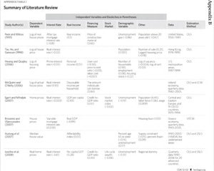
Many scholars have found that home prices are affected by the real after-tax interest rate, permanent income, mortgage credit, the vacancy rate, the distribution of income, the unemployment rate, the price-to-income ratio, annual growth in home prices, financial deepening, and demographic factors such as percentage of the population age 65 or older and changes in household size. Regardless of the methodology used, many studies have found a negative correlation between home prices and interest rates. In addition, some have concluded that interest rates cannot explain a large part of home price movements, and a few have found that down payment changes are unlikely to have a major impact on home prices.
Joe Peek and James Wilcox use data from 1950 to 1989 to estimate home prices as a function of unemployment rates, financing costs, demographic factors, and material costs within the framework of a reduced form equation derived from supply and demand functions. The supply depends on real house prices and the price of construction materials. The demand is positively related to the real income, size, and age distribution of the population and negatively related to real house prices, unemployment rate, and homeowners’ real after-tax borrowing costs. Using ordinary least squares (OLS), they find that real home prices are negatively correlated with the real after-tax interest rate and positively correlated with permanent income and cost of materials. Demographic factors such as age and distribution of income are also among significant determinants of home prices.[11]
Raymond Tse, C. W. Ho, and S. Ganesan use the data on Hong Kong real estate markets to estimate the determinants of home prices. They use a reduced form equilibrium model to explain changes in house prices by variables such as nominal interest rate, changes in consumer price index, and transactions volume. Their results indicate that these variables can fully explain home prices.[12]
Min Hwang and John Quigley use U.S. metropolitan data over a 13-year period (1987–1999) and develop a model that relates variables such as regional employment, income, construction costs, vacancy, and new construction to housing market prices. Their result highlights the importance of income and employment in real home prices.[13]
Lance Freeman and his colleagues use an econometric analysis to test whether GSE activities lead to better housing market conditions. They study the secondary mortgage market across underserved areas in Cleveland, Ohio, from 1993 to 1999 and find no significant relationship between mortgage interest rates and home prices after controlling for a variety of neighborhood characteristics.[14]
Kieran McQuinn and Gerard O’Reilly use quarterly data for 1980 to 2005 and variables such as disposable income, interest rate, house prices, and amount borrowed for the Irish economy. They use dynamic OLS to estimate the relationship between house prices and interest rates and find that shifts in home prices can be explained by the amount an individual can borrow from financial institutions, disposable income, and the interest rate.[15]
Balázs Égert and Dubravko Mihaljek investigate the determinants of home prices in 19 Organisation for Economic Co-operation and Development (OECD) countries from 1975 to 1994 and in transition economies in Central Eastern Europe (CEE) between 1993 and 1998. They use gross domestic product (GDP) per capita, the real interest rate, the equity price index, the unemployment rate, population, and the share of labor force in the population as independent variables. They find that fundamentals play an important role in shaping home prices in both OECD and CEE countries. However, they find a robust relationship between home prices and interest rates.[16]
Sophocles Brissmis and Thomas Vlassopoulos investigate the interactions between mortgage financing and home prices in Greece. They use quarterly data from the fourth quarter of 1993 to the second quarter of 2005 and variables such as the amount of the housing loan, GDP, the mortgage interest rate, and residential property prices. Using a vector error correction model (VECM), their results suggest that housing prices are weakly exogenous in the long run, meaning that the causality is not from housing loans to home prices. However, their short-run analysis indicates a contemporaneous bidirectional dependence between housing loans and home prices.[17]
An Xudong, Raphael Bostic, Yongheng Deng, and Stuart Gabriel conduct two tests to evaluate the effects of GSE mortgage purchases on median house value and homeownership rate. They use data from 1990 to 2000 and test the hypotheses that GSE performance in targeted areas affects home prices. They use a list of sociodemographic characteristics and such independent variables as the price-to-income ratio, the annual growth in home prices, the supply constraint index, the percentage of the population age 65 or older, changes in household size, the change in minority percentage of the population, and the unemployment rate. They find that increased GSE activity is statistically associated with declines in neighborhood vacancy rates and increases in median home value.[18]
Iossifov Plamen, Martin Cihak, and Amar Shanhavi use quarterly data for 20 advanced countries from 1990 to 2006 to find the determinants of home prices. Their independent variables are life-cycle wealth, the short-term interest rate, the spread between long-term and short-term interest rates, inflation, the unemployment rate, a measure of financial deepening, and demographic variables such as the share of active population, the total population, the government balance as a ratio of GDP, and the current account balance as a ratio of GDP. Their results suggest that the elasticity of residential housing prices to the short-term interest rate is –3.6.[19]
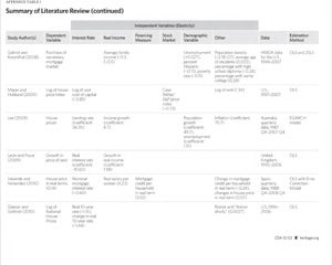
Stuart Gabriel and Stuart Rosenthal use data from the Housing Mortgage Data Agency (HMDA) from 1994 to 2008 for conventional loans. They find that GSE crowding-out effects were small prior to 2002, when private lenders held a noticeable share of the market. However, this crowding-out effect on private market activity was substantial during the housing boom of 2003–2006.[20]
Christopher Mayer and Glenn Hubbard implement a user-cost model for housing prices and variables such as the ratio of rent to income as a measure of housing affordability, the after-tax interest rate, the equivalent risk opportunity, the cost of capital, expectations of future home price appreciation, and the Case and Shiller/S&P house price index to determine whether home prices overshoot their fundamentals. Using data from 1950 to 2000, they find that declines in the interest rate can explain the super-normal rates of home price appreciations in “superstar cities,” such as Boston, Los Angles, New York, and San Francisco. In summary, their results suggest that the real interest rate has an important impact on home prices.[21]
Chyi Lin Lee uses an EGARCH model for eight large cities in Australia using data from the fourth quarter of 1987 to the last quarter of 2007 to investigate the determinants of home prices. His list of variables is the Consumer Price Index, personal income, population, and the unemployment rate. He finds that inflation is the most important determinant of home price volatility at the national level.[22]
Eric Levin and Gwilym Pryce use data from 1996 to 2006 for the economy of the United Kingdom and investigate the effects of the rent-to-price ratio and long-term real interest rate on home prices. They conclude that the decline in the long-term real interest rate has contributed to the rising home prices. They argue that cyclical asymmetries inherent in the supply of real estate have been exacerbated by changes in the financial system and increased government regulation.[23]
Santiago Valverde and Francisco Fernandez use quarterly data for the fourth quarter of 1988 through the fourth quarter of 2008 to analyze the relationship between home prices and mortgage credit in Spain. They use the vector-error correction model and such variables as the price-to-rent ratio, mortgage credit per household in real terms, and real salary per worker. They find that house prices in Spain are mainly affected by mortgage lending.[24]
Edward Glaeser, Joshua Gottlieb, and Joseph Gyourko use data from 1980 through 2008 for the U.S. and variables such as the mortgage interest rate, the Treasury bill rate, the loan approval rate, the loan-to-value ratio, the Case and Shiller Index, and the Romer and Romer shock index. They find that interest rate plays a trivial role in explaining housing prices. They also find that down payment changes are unlikely to have a major impact on home prices. They conclude that interest rates influence home prices, but they cannot explain a large part of the movement in home prices. Neither the approval rate nor the down payment requirement can explain most or a major part of the movement in home prices. However, they find that the number of applications and the nature of new borrowers contributed to the booms.[25]
Theoretical Model
A reduced form equation for the real home prices can be obtained from the models of aggregate supply and demand for real estate markets. The liquidation of Fannie Mae and Freddie Mac is expected to affect home prices through two main channels—mortgage interest rate and down payment requirement—because the GSEs have been involved in practices that mainly affect these two variables. Indeed, in 1996, Fannie Mae and Freddie Mac eased the requirements for down payments and started to subsidize mortgage interest rates for purchasing a house.
This analysis extends the seminal study of Peek and Wilcox,[26] acknowledging that the demand for real estate depends negatively on the home price (HP), the conventional 30-year mortgage interest rate (Mr30),[27] the down payment (Dpayment), the unemployment rate (Unemp), rent as a substitution for purchasing a house (Rent), and the term structure of a mortgage loan (term). Demand for real estate also depends positively on household assets (Hassets), personal income (Perincome), and inflation expectations for home prices (Inf).

On the supply side, the stock of houses responds positively to home prices and negatively to the vacancy rate (vacancy) and property taxes (proptax).[28] A higher property tax rate reduces the incentives for investment and, as a result, reduces the supply of home stock.

As Glaeser et al. conjecture in the classic asset market approach, down payment level does not matter because home buyers are indifferent between paying cash and borrowing.[29] In other words, in the classic asset market approach, buyers discount at the market rate and are not credit constrained. However, in the real world, down payment level does matter because buyers are credit constrained and like to borrow at the market rate. Therefore, any changes in down payment requirements could change home prices. The analysis assumes that buyers are homogenous, so the characteristics of a marginal buyer remain unchanged when the down payment rises due to the liquidation of GSEs.
Any change in down payment requirement is believed to affect home prices through two channels:
- First, a higher down payment reduces the affordability to the buyer if the buyer is budget constrained and thus reduces the demand for real estate. Therefore, a negative effect on home prices is expected.
- Second, a higher down payment provides more resources to financial institutions, which positively affects the amount of available mortgage loans to potential home buyers.
Assuming that these resources will be available to new home buyers, it stimulates the demand side and leads to higher home prices. Thus, there are two different channels operating in opposite directions. The first channel is an income effect, and the second is a substitution effect. The final impact on home prices depends on which channel dominates.

Data
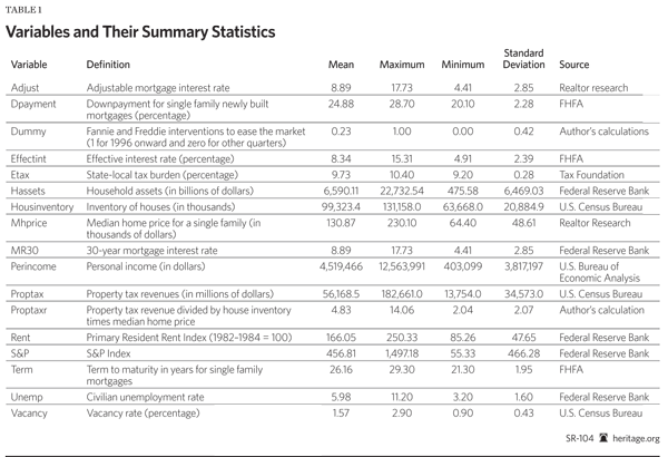
The analysis uses quarterly data from the first quarter of 1980 to the last quarter of 2010 to estimate the effects of changes in mortgage interest rates and down payments on median home prices. The variables, their summary statistics, and their sources are presented in Table 1. The data on vacancy rate, house inventory, and property tax revenues were obtained from the Census Bureau. The data on down payments, effective interest rate, and term structure were retrieved from the Federal Housing Finance Agency (FHFA). Data on adjustable mortgage interest rates and median home prices are from Realtors Research. The data on tax burden rate were retrieved from the Tax Foundation. The rest of the variables were retrieved from the Federal Reserve Bank of St. Louis, except personal income, which was obtained from the Bureau of Economic Analysis in the U.S. Department of Commerce.
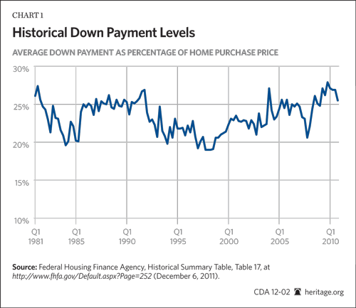
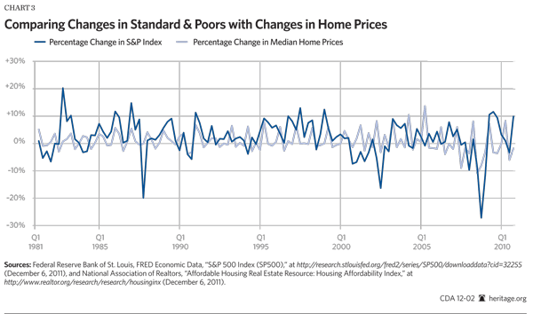
Stylized Facts in the U.S. Housing Market. An important stylized fact—a simplified presentation of an empirical finding—in the U.S. housing market is that down payments have been relatively stable over time, but home prices have been volatile, increasing until the third quarter of 2006 and then dropping off sharply. The data suggest that down payments have not played an important role in shaping peaks and troughs in the housing market because they have been relatively stable, varying between 20 percent to 28 percent at the national level, whereas the median home price has been relatively volatile over time (see Chart 3), underlining that there is no significant relationship between the two.
Later on, the analysis tests the hypothesis that prices are inelastic to down payments in the econometric section. If home prices are inelastic to down payments, this implies that GSE interventions in the market to ease the access to loans among home buyers have not significantly affected home prices. Therefore, liquidating GSEs may affect home prices only marginally or not at all. This corollary has important policy implications because it can pave the way for a housing market without GSEs.
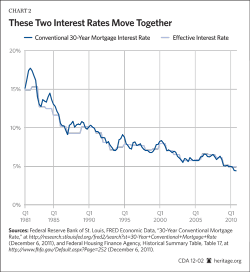
Another stylized fact is that the conventional 30-year mortgage interest rate and effective interest rate have moved together very closely since 2003, suggesting that most loans are dominated by the conventional 30-year mortgage interest rate rather than by market interest rates. (See Chart 2.) Indeed, the intervention of the giant monopolies has been so intense that most loans have a subsidized interest rate.
Finally, changes in home prices and the S&P Index have been moving closely together (see Chart 3), although the S&P Index has higher volatility, especially during the sharp drops in 1987 and 2008. The analysis tests the hypothesis that the S&P Index has played any role in explaining median home price in the econometric section. Indeed, the S&P Index is anticipated to affect real estate prices through two channels:
- People look at real estate as an alternative to investing in the stock market, suggesting a negative correlation between the S&P Index and home prices.
- The two may be positively correlated because household assets inflate when the stock market index soars. This, in turn, induces demand for real estate and leads to higher home prices.
Econometric Results. In this section, the reduced form equation described in the theoretical section is estimated. This study examines the elasticity of median home prices at the national level to the conventional 30-year mortgage interest rate and down payments after accounting for such fundamentals as household assets, personal income, the unemployment rate, property taxes, the vacancy rate, and inflation expectations of home prices.
Table 2 summarizes the estimated OLS results for housing prices at the national level for six model specifications. The models use different indexes for mortgage interest rates, including the conventional 30-year mortgage interest rate, the adjustable mortgage rate, and the effective mortgage interest rate, to determine whether the results are still robust. In addition, three different tax rates have been embedded into the models: the effective tax burden rate issued by the Tax Foundation, tax revenues in millions of dollars reported by the Census Bureau, and the property tax rate calculated by dividing tax revenues (the nominator) by median home prices and home inventories (the denominator). All models are estimated in log form; therefore, the coefficients are elasticities.
Model 1 indicates that the coefficient on the conventional mortgage interest rate is negative, as expected, and statistically significant at the P = 0.05 level. Indeed, the elasticity of median home price to conventional mortgage interest rate is as low as –0.09 in Models 1, 5, and 6. Assuming a 25-basis-point increase in the conventional mortgage interest rate as a result of GSE liquidation as discussed in the literature and in the President’s budget for fiscal year 2012,[30] holding other things equal, leads to a 2.25 percent reduction in home prices. In other words, a jump in interest rates of 25 basis points has a marginal negative impact on home prices. Therefore, liquidating GSEs will likely not lead to higher home prices.
Model 2 captures the effects of the adjustable mortgage interest rate rather than the 30-year conventional mortgage interest rate on median home prices. The results indicate that the elasticity of the median home price to adjustable mortgage interest rate is as low as –0.03 and not statistically significant. Model 3 captures the effects of effective interest rate rather than mortgage interest rate. The coefficient on this variable is –0.07 and not statistically significant. Therefore, the most significant variable in shaping home prices is the conventional mortgage interest rate.
The down payment coefficient is negative, as expected, and equals –0.06 when using the property tax rates in Model 6. This result indicates that a 25-basis-point increase in down payment leads to a 1.5 percent reduction in home prices. In summary, the results suggest that prices are more elastic to mortgage interest rate than down payments are. This has important implications for financial institutions because changing the down payment compared to the mortgage interest rate will have less impact on home prices.
Following Mayer and Hubbard,[31] the S&P Index has been embedded into Model 4 to determine whether the stock market index can explain the volatility of home prices. The results indicate that the S&P Index coefficient is positive, as expected, and statistically significant at P = 0.5. In other words, a 10 percent rise in the stock market index leads to a 0.5 percent increase in median home price.
The coefficient for effective tax burden is statistically significant and positive, as expected, and ranges from 0.46 to 0.62, meaning that a 10 percent increase in the tax burden will lead to a 4.6 percent to 6.2 percent increase in home prices. However, if the property tax revenue collected by the government or the property tax rate is used, the coefficient changes to negative, although it is still statistically significant. This result is due to the lack of solid quarterly data on the property tax rate per square foot for the period under investigation.[32]
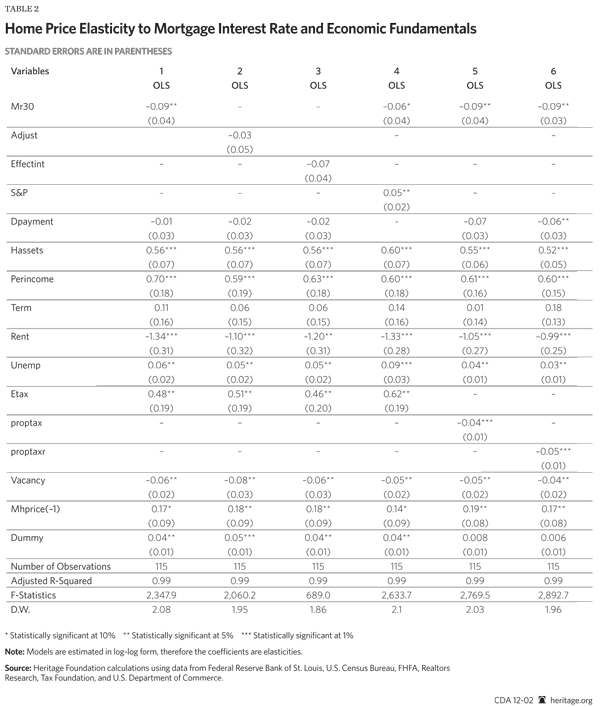
Interestingly, both household assets and personal income have positive and significant effects on home prices in all models. Indeed, household assets and personal income are the most important factors in shaping home prices in this model. While a 10 percent increase in household assets leads to a 5.6 percent to 6.0 percent increase in home prices, a 10 percent increase in personal income leads to a 5.9 percent to 7.0 percent increase in home prices, underlining that personal income matters more than household assets in shaping home prices.
Another important factor in shaping home prices is the expectation of future home price appreciation, which is measured by previous-period home value. The results suggest that the coefficient is positive and statistically significant at p = 0.05 level in Models 2, 3, 5, and 6. In other words, a 10 percent increase in the expected inflation of home value leads to a 1.4 percent to 1.9 percent increase in home prices.
The analysis also uses a dummy variable for the periods during which Fannie Mae and Freddie Mac eased the requirements for purchasing a house (i.e., the first quarter of 1996 and every subsequent quarter are input as a 1, and every preceding quarter is a zero) and finds that this variable is statistically significant at p = 0.05 except in Models 5 and 6. Contrary to policymakers’ expectations, the coefficient is positive, indicating that home prices have increased due to GSE interventions in the housing market. Therefore, the analysis implicitly suggests that the homeownership rate should have decreased due to higher prices. This effect will be considered in a forthcoming Heritage Foundation study.
The Durbin–Watson statistics suggest that all models are robust relative to autocorrelation. In other words, residuals from OLS regression are not autocorrelated at the P = 0.05 significance level.[33]
In summary, the results indicate that home prices are affected mainly by fundamentals, such as household assets, personal income, the S&P Index, and the effective tax rate. The results also suggest that the unemployment rate has a statistically significant impact on home prices in all models, although the opposite of the expected sign. In other words, a 10 percent rise in unemployment leads to a 0.3 percent to 0.9 percent increase in home prices. The reason for the positive sign may be biased data on the unemployment rate, which do not capture the total unemployed population, particularly those who have given up searching for a job. Alternatively, the economy may be staying on the upward trend of non-accelerating inflation rate of unemployment (NAIRU), experiencing a higher unemployment rate with higher prices, including home prices.
These results are consistent with Glaeser et al.,[34] who find that the interest rate plays a minimal role in explaining home prices and that down payment requirements are unlikely to have a major impact on home prices. Finally, the results also suggest that GSE intervention in the market has led to higher home prices, contrary to policymakers’ expectations.
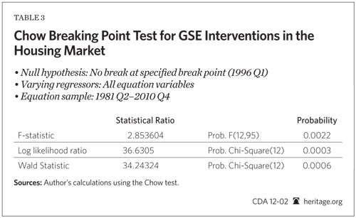
This analysis also performed the Chow breaking point test, instead of dummy variable, to determine whether GSE intervention in the market since 1996 has significantly affected home prices. The result, presented in Table 3, rejects the null hypothesis of no breaking point, strengthening the case that the GSE interventions since 1996 have led to higher home prices.
Conclusion
Clearly, the results of this analysis, which are consistent with many other empirical studies, suggest that interest rates influence home prices but cannot provide anything close to a complete explanation of real estate market behavior during 2003–2010. Our results suggest that neither down payments nor mortgage interest rates are substantial determinants of home prices. However, fundamentals—such as household assets, personal income, the S&P Index, and the effective tax rate—play substantial roles in shaping home prices.
The results of our analysis are in line with those of Freeman et al., who find no evidence supporting the idea that variations in GSE mortgage interest rates are significantly and positively associated with changes in home prices.[35] Our results are also consistent with those of Glaeser et al., who find that changes in down payment requirements and interest rates are unlikely to have a major impact on home prices.[36]
The coefficient on the dummy variable for measuring GSE intervention in the housing market suggests that the interventions have led to higher prices by increasing demand through easy access to mortgage credit, which may have adversely affected poor and low-income groups. Therefore, if the federal government plans to improve the housing market in underserved areas, it should consider other policy instruments rather than subsidizing mortgage interest rates or easing down payment requirements, which have failed to achieve its housing market goals.
Policy Discussion
The federal government’s policy of subsidizing mortgage interest rates and lowering down payments to raise homeownership has failed due to inelasticity of home prices to these variables. The results of this study cast doubt on the effectiveness of the GSE interventions in the housing market through subsidizing interest rates and lowering down payment requirements because these variables do not play major roles in shaping home prices.
In essence, the government intervention has led to a large deadweight loss for society rather than helping low-income individuals to secure homeownership through lower prices. Although lower interest rates through a macroeconomic stimulus package may benefit borrowers who refinance existing mortgages at lower interest rates for a while, market imperfections and asymmetric information may prevent this from having a long-term benefit.
The results of this study have important implications for policymakers. The federal government should avoid offering any subsidy in the form of lower interest rates or lower down payments because it adversely affects both the housing market and the economy over the long term. Although such a policy may boost the demand side in the short term, it risks inflating another housing bubble in the medium or long term.
The appropriate action is to reestablish market forces by phasing out GSEs. Although GSE supporters may argue that diluting these two corporations would lead to higher interest rates for borrowers, our econometric results indicate that higher interest rates will lead to lower median home prices, which in turn will increase the ability of low-income groups to purchase a house. Moreover, elimination of GSEs will enhance competition among financial institutions, leading to lower interest rates in the medium to long term. Curtailing the monopolies in the housing market will certainly contribute to achieving housing market goals and reducing the large amounts of deadweight loss.
—Nahid Kalbasi Anaraki, Ph.D., is a Visiting Fellow for Special Projects in the Center for Data Analysis at The Heritage Foundation.
Appendix A
Fannie Mae and Freddie Mac Interventions in the Housing Market
| 1975 | Risk regulators, with secondary adoption of National Recognized Statistical Rating Organizations (NRSROs), begin moving from “prudent” to risk-based rating. |
| 1986 | Real Estate Mortgage Investment Conduits (REMICs), introduced by the Tax Reform Act of 1986, encourage private securitization by allowing credit tranches into subordinate securities. Opposition from the newly privatized Freddie Mac and long privatized Fannie Mae prevent private securitization from being established. |
| 1992 | Federal Housing Enterprise Financial Safety and Soundness Act establishes the Office of Federal Housing Enterprise Oversight (OFHEO) as a regulator. |
| 1995 | HUD gives target goals to Fannie and Freddie to raise homeownership rate among low-income groups. The Administration raises the homeownership rate goal to 70 percent. |
| 1999 | Fannie Mae eases the requirements on loans and moves to subprime mortgages. |
| 2004 | HUD urges Fannie and Freddie to increase their purchases of subprime and Alt-A (between prime and subprime) mortgages. |
| May 2007 | The House passes Federal Housing Finance Reform Act of 2007, which would create a new regulator, but with no control over the mortgage-backed securities portfolios of Fannie and Freddie. |
| July 2008 | When the Fannie and Freddie reach the financial precipice, the House and Senate pass the Federal Housing Finance Regulatory Reform Act of 2008. |

